WIKI Calcium imaging analysis using biophysical models
- Calcium imaging
- CaBBI: A novel method for calcium imaging analysis
- CaBBI demos step by step
- Want to adapt CaBBI demo scripts to your own data?
- References
This page describes the demo codes of CaBBI (Rahmati et al. 2016), which is a novel method for analyzing (deconvolving) calcium imaging data. More precisely, CaBBI infers neuronal dynamics and parameters from calcium imaging data. For an example of implementation, see the demo_CaIBB_FHN and demo_CaIBB_QGIF functions.
Calcium imaging
Calcium imaging was designed to monitor the neuronal activity of both individual neurons and neuronal populations. Calcium imaging data are fluorescence traces that encode the change in (intracellular) calcium concentration ([Ca2+]). The firing activities are encoded as fluorescence transients, composed of (usually) a rising phase and a decaying phase. In brief, when a neuron fires, [Ca2+] elevates (rising phase) due to the opening of voltage-gated calcium channels (mainly L-type channels), which allows for Ca2+ influx to the cytoplasm. This initial increase is then decayed exponentially by removal mechanisms such as pumping and buffering (decaying phase).
CaBBI: A novel method for calcium imaging analysis
Typically, one wants to reconstruct firing activity (e.g., spike trains) from fluorescence traces. However, this is not a trivial problem because data is polluted by noise, it has low temporal resolution (in regular recording configurations), and there is an indirect nonlinear relationship between [Ca2+] kinetics and the underlying membrane potentials.
In Rahmati et al. (2016), a new method called CaBBI (Calcium imaging analysis using Biophysical models and Bayesian Inference) was proposed. CaBBI is based on a biophysical generative models of fluorescence data (see Figure below) that includes both evolution and observation mappings. The evolution function governing the dynamics of spiking states, calcium channels, and [Ca2+] kinetics. The generated [Ca2+] kinetics are then mapped non-linearly to the fluorescence kinetics through the observation equation. These mappings are used to recover the hidden states given a measured fluoresce trace (through VBA model inversion). This method has several remarkable advantages over standard methods such as “template matching” and other agnostic machine learning methods:
- First, CaBBI incorporates biophysical mechanisms of spike and/or burst generation, by using the spiking and bursting neuron models. Using such priors allows for a much more reliable inference about firing events.
- Second, it can intrinsically be adapted to fluorescence transients with different rise and/or decay times. In particular, it can even reconstruct the firing events from relatively slowly rising fluorescence transients, as with new genetically-encoded calcium indicators.
- Third, CaBBI not only reconstructs the firing patterns, but also estimates interpretable biophysical states such as membrane potential, [Ca2+] kinetics, and some voltage-gated currents/conductances.
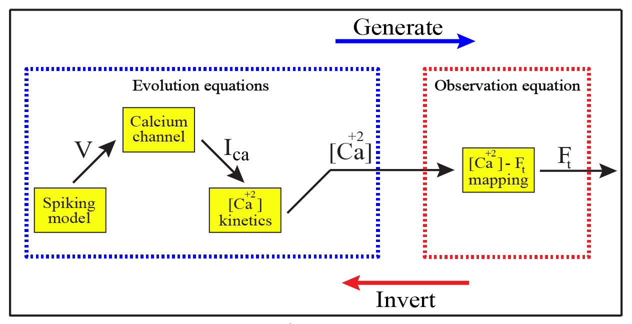
Schena of the CaBBI Graph illustrating CaBBI’s generative model and its inversion. The represented hierarchy in the graph displays how neuronal dynamics relate to fluorescence traces.
CaBBI can be used with different spiking models. In Rahmati et al. (2016), authors demonstrate the well-known Fitzhugh-Nagumo (FHN) model and the so-called “Quadratic-Gaussian Integrate-and-Fire model” (QGIF), which does not require any reset condition (neither for producing the upstroke phase of the spike nor for its re-polarization phase).
CaBBI demos step by step
The demonstration scripts demo_CaIBB_FHN and demo_CaIBB_QGIF show how to invert the FHN and QGIF generative models, respectively, given a measured fluorescence trace. By default, the demonstration scripts automatically download the clacium imaging data that was processed in Rahmati et al. (2016). These in-vitro data were recorded from neonatal hippocampal tissues with a sampling rate of 22.6 Hz. Note that the ensuing fluorescence transients have relatively very slow rising phases, which render model inversions particularly difficult. This is why recorded data are pre-processed (slow temporal drifts removal) prior to model inversion.
The Figure below is an example of the graphical output of demo_CaIBB_FHN:
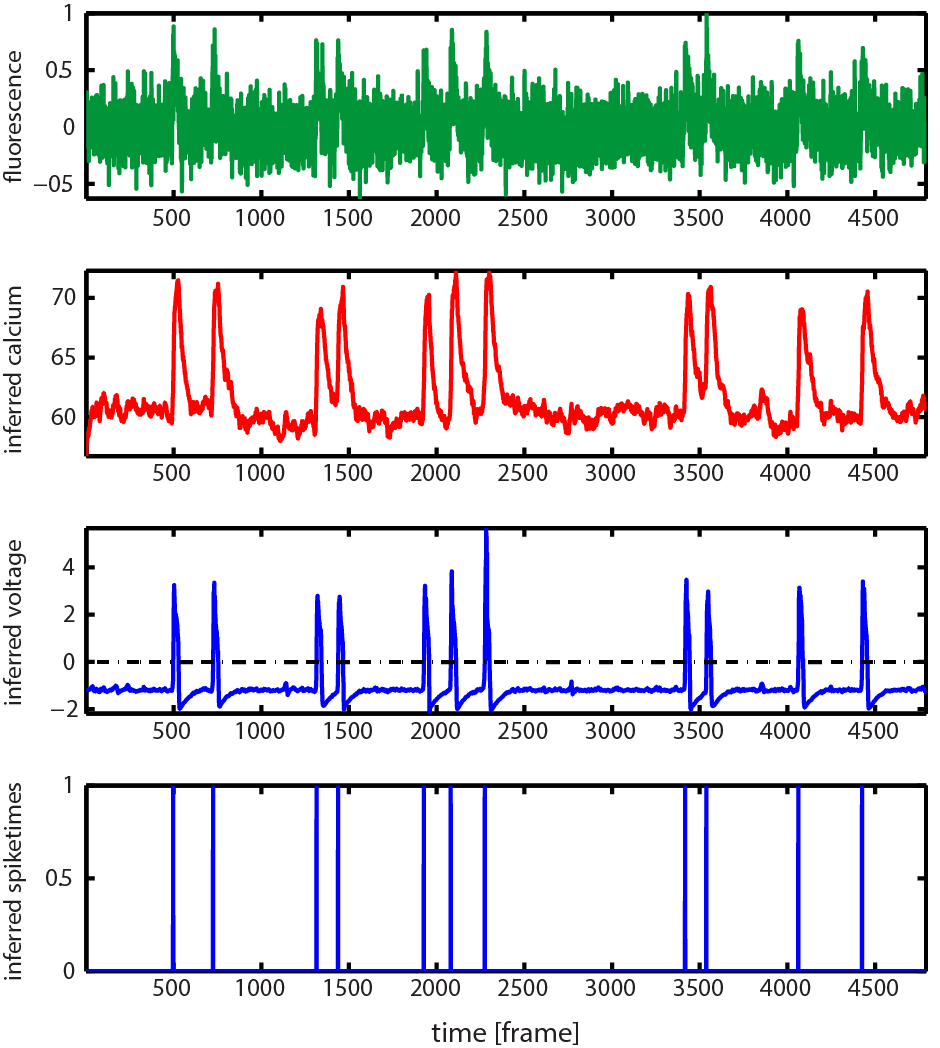
First row: the pre-processed fluorescence trace, Second row: estimated [Ca2+] kinetics, Third row: estimated membrane potentials, Fourth row: estimated spiking event times (obtained by thresholding the inferred membrane potentials, see Step 9 below). Note: all these variables are automatically saved in
CaBBI.
Below, we comment the demonstration scripts step by step:
- Step 1: The downloaded data contains eight traces: pick the trace you want, e.g.:
% file name of the fluorescence trace Fluor_trace_name = 'fluorescence_data7'; - Step 2: specify the sampling rate (in Hz) of the fluorescence trace:
sampling_rate = 22.6; - Step 3: polynomial de-trending method (low frequency drift removal). You can select the degree of the polynomial (either 3 or 4) which will be fitted to the data, e.g.:
% Polynomial degree (4 or 3) degree = '4'; - Steps 5 to 7: Specify VBA inversion options (including priors).
nFrames = numel(Fluor_trace); % number of recording frames dt = 0.2; % [ms], time step size of the FHN model inF.dt = dt; inF.k_Ca0 = 0.002; % scale parameter of [Ca2+] kinetics TauCa_realTime = 7500; % [ms], the prior for decay time-constant of calcium transients in real time dt_real = 1000/sampling_rate; % [ms], frame duration (temporal precision) of fluorescence data inF.Tau_Ca0 = TauCa_realTime*dt/dt_real; % effective prior mean of tau_Ca in inversion; see Eqn. 17 inG.k_F0 = 5; % scale parameter of the fluorescence observatios inG.ind = 3; % index of [Ca2+] variable options.inF = inF; options.inG = inG; - Step 8: VBA inversion of the FHN model given the observed fluorescence trace:
f_fname = @f_CaBBI_QGIF; % CaBBI evolution function [depends upon the CaBBI demo script] g_fname = @g_CaBBI; % CaBBI observation function u = zeros(1,numel(Fluor_trace)); % dummy system's input dim.n = 3; % number of states dim.n_phi = 2; % number of observation params dim.n_theta = 3; % number of evolution params [posterior, out] = VBA_NLStateSpaceModel(Fluor_trace,u,f_fname,g_fname,dim,options); -
Step 9: Extracting the estimated Voltage and [Ca2+] traces (i.e. the posterior means on hidden states)
- Step 10: Detecting spike times (or event onsets) from inferred voltage trace.
To deal with neural noise, an artificial refractory period is enforced after each detected spike event (i.e. all up-crossing fluctuations within the refractory period will be discarded). You can specify this refractory period by modifying the following lines of code:
refracPeriod = 6; % here: 6 msec if (count > 1) && ( (j-indices(count-1)) > ceil(refracPeriod/dt) ) ... - Step 11: save the variables of interest. For example, the estimated decay time-constant of the calcium transients (see also Eq. 17 in Rahmati et al. 2016) can be accessed as follows:
% in [sec]
inferred_Tau_Ca = inF.Tau_Ca0 * exp(posterior.muTheta(1)) * (1/sampling_rate)/dt
Want to adapt CaBBI demo scripts to your own data?
Simply specify the directory where your fluorescence trace is saved, as well as your data sampling rate (in Hz). Running the demo scripts will automatically remove the low frequency drifts from your data, and invert the corresponding generative model. The parameters and states estimates will be stored in CaBBI (see Step 11).
References
Author: Vahid Rahmati, (vahidrahmati92@gmail.com)