WIKI Neurobiological models
Dynamic Causal Modelling of fMRI data
Decomposing the relation existing between cognitive functions and their neurobiological “signature” (the spatio-temporal properties of brain activity) requires an understanding of how information is transmitted through brain networks. The ambition here is to ask questions such as: “what is the nature of the information that region A passes on to region B”? This stems from the notion of functional integration, which views function as an emergent property of brain networks. Dynamic causal modelling –DCM- has been specifically developed to address this question.
Dynamic Causal Modelling or DCM embraces a graph-theoretic perspective on brain networks, whereby functionally segregated sources (i.e. brain regions or neuronal populations) correspond to “nodes” and conditional dependencies among the hidden states of each node are mediated by effective connectivity (directed “edges”). DCM generative models are causal in at least two senses:
- DCM describes how experimental manipulations influence the dynamics of hidden (neuronal) states of the system using ordinary differential equations. These evolution equations summarize the biophysical mechanisms underlying the temporal evolution of states, given a set of unknown evolution parameters that determine both the presence/absence of edges in the graph and how these influence the dynamics of the system’s states.
- DCM maps the system’s hidden states to experimental measures. This observation equation accounts for the main characteristics of the neuroimaging apparatus.
The inversion of such models given neuroimaging data can then be used to identify the structure of brain networks and their specific modulation by the experimental manipulation (i.e. induced plasticity). For example, showing that a given connection is modulated by the saliency of some stimulus demonstrates that this connection conveys the saliency information.
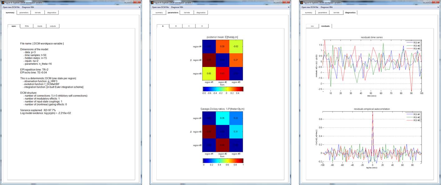
SPM proposed the seminal software implementations of DCM. The following script allows one to invert an SPM-specified DCM model using VBA, and then eyeball inversion results and diagnostics:
[y,u,f_fname,g_fname,dim,options] = dcm2vba(DCM);
[posterior,out] = VBA_NLStateSpaceModel(y,u,f_fname,g_fname,dim,options);
DCM = vba2dcm(posterior,out,[],TR);
spm_dcm_explore(DCM)
where DCM is the variable saved in the SPM DCM-file and TR is the fMRI repetition time.
A number of demonstration scripts have been written for DCM:
demo_dcm_1region.m: this script simulates and inverts a 1-node network model. It is useful to assess the statistical identifiability of local self-inhibitory processes and neuro-vascular coupling parameters.demo_dcm4fmri.m: this script simulates and inverts a 3-nodes network model, with induced network plasticity. Emphasis is put on the influence of neural noise on the system’s dynamics.demo_dcm4fmri_distributed.m: this script simulates and inverts a 3-nodes network model (same as above). Here, the observation function has been augmented with unknown spatial profile of activation, which can be useful to capture non-trivial spatial encoding of experimentally controlled stimuli or observed behaviour.
Neural fields
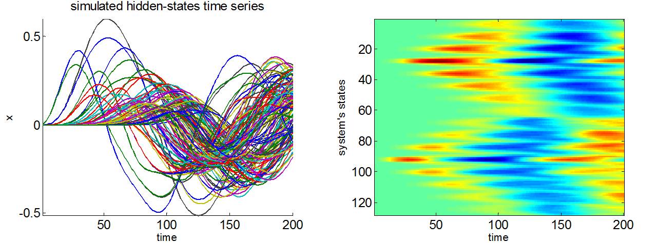
These models are inspired from statistical physics approaches based upon the notion of mean field, i.e. the idea that interactions within micro-scale ensembles of neurons can be captured by summary statistics (i.e., moments of the relevant distribution). They describe the spatio-temporal response of brain networks to experimental manipulations.
At this macroscopic scale, neural states like mean membrane depolarisation can be regarded as a continuum or field, which is a function of space and time. The spatiotemporal dynamics of neural fields essentially depend on how local ensembles influence each other, through connectivity kernels. The latter quantify the amount of anatomical connections as a function of physical distance between any two points on the field. We refer the interested reader to the demonstration script demo_2DneuralField.m.
Spiking neuron models
This class of models attempt to capture how individual neurons respond to inputs, typically in terms of ion currents that flow through the cell membrane (this occurs when neurotransmitters cause an activation of ion channels in the cell).
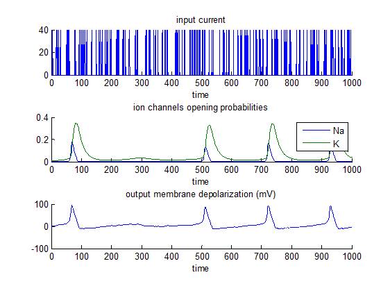
Hodgkin-Huxley model
This is the most established model of spiking neurons, which was developed from Hodgkin and Huxley’s 1952 work based on data from the squid giant axon. In brief, short bursts of depolarizing input current are sent to a neuron that has a all-or-none response if the membrane depolarization reaches a critical threshold (approx. 80mV). The script demo_HH.m simulates the response of such a neuron, and then inverts the model. Emphasis is put on the identifiability of model parameters (e.g. K/Na conductances).
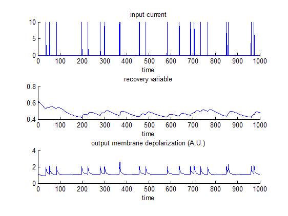
Fitzhugh-Nagumo model
This is essentially a reduction of the Hodgkin-Huxley model, which was introduced by FitzHugh and Nagumo in 1961 and 1962. In brief, the model captures the neuron’s “regenerative self-excitation” using a nonlinear positive-feedback membrane voltage, as well as its recovery dynamics using a linear negative-feedback gate voltage. Note that this does not generate ‘all-or-none’ spikes (as in the Hodgkin-Huxley model), but supra-threshold input create large deviations from equilibrium membrane depolarization. NB: an AP approximately corresponds to a deviation of about 1 A.U. w.r.t. equilibrium. The script demo_FHN.m simulates the response of such a neuron, and then inverts the model. Emphasis is put on the identifiability of model parameters (e.g. recovery time constants). In contradistinction, the script demo_fitzhugh.m assesses whether one can use VBA’s stochastic inversion to identify the system’s input.