WIKI Statistical models
- Classical GLM data analysis
- 1D-RFT: solving the multiple comparison problem with Random Field Theory
- GLM with missing data
- Mediation analysis
- Binary data classification
- Kalman filter/smoother
- Probabilistic clustering
Classical GLM data analysis
The general linear model (GLM) is a statistical linear model that relates a dependent variable \(y\) to a linear combination of independent variables \(X\) as follows:
\[y = X \beta + e\]where \(e\) are model residuals, \(\beta\) are unknown regresion coefficients and \(X\) is the so-called design matrix. GLMs of this sort are equivalent to “multiple regression models”, and typical questions of interest can be framed in terms of a contrast of independent variables. This is equivalent to testing for the significance of \(c^T \beta\), where \(c\) is the contrast vector or matrix. Inference on such contrasts in the context of a GLM is very general, and grand-fathers most classical statistical approaches, including ANOVA, ANCOVA, MANOVA, MANCOVA, ordinary linear regression, t-test and F-test.
Let us consider a toy example, where the GLM reduces to four dependant (and, here, arbitrary) variables \(X_i\) (where \(i=1,...,4\)). We simulate dummy data where only the first dependant variable actually induces variability across the 32 samples of the dependant variable \(y\), and then use the function GLM_contrast.m to perform classical inference on the contrast of interest:
X  = randn(32, 4); % simulate dummy independent variables
b  = [1.5; 0; 0; 0 ]; % only the first independent variable has an effect
y  = X*b; % simulate the dependent variable under the GLM
y  = y + randn(size(y)); % add random noise
c  = [1;0;0;0]; % contrast vector --> testing for the first independent variable
type = 'F'; % use F-test
pv = GLM_contrast(X, y, c, type); % classical hypothesis testing
where c is the contrast matrix, type is a flag for the test (t-test or F-test) and pv is the p-value of the corresponding test (in this example, the contrast effectively tests for the significance of the first regressor of the design matrix).
Let us eyeball the graphical output of the function GLM_contrast.m:
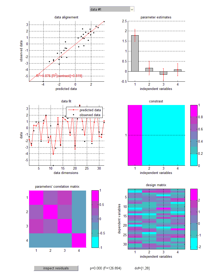
Upper-left panel: observed data (y-axis) plotted against predicted data (x-axis). NB: The total percentage of explained variance is indicated (\(R^2\)), as well as the percentage of variance explained by the contrast of interest. Middle-left panel: observed and predicted data (y-axis) plotted against data dimensions (x-axis). Lower-left panel: parameter’s correlation matrix. Upper-right panel: GLM parameter estimates plus or minus one standard deviation. NB: Right-clicking on barplots allows one to access the results of individual significance F-tests. Middle-right panel: contrast of interest. Lower-right panel: design matrix. Note: some GLM diagnoses (e.g., normality and homoscedasticity of model residuals) can be eyeballed (cf. “inspect residuals” at the bottom of the figure).
Note that t-tests effectively perform one-tailed tests (positive effects). This means that the sign of the contrast matters. In contradistinction, F-tests perform two-tailed tests.
The function GLM_contrast.m can output more than just the p-value. In fact, all descriptive statistics can be retrieved from optional output arguments to GLM_contrast.m. In particular, it can be used to recover ordinary least-squares (OLS) estimates of GLM parameters and residual variance, as well as summary statistics such as t- or F- values and percentages of explained variance…
Tip: defining contrasts for, e.g., main effects of multi-level factors can be tedious. However, VBA has an in-built function for doing exactly this:
Contrast_MEbins.m. It outputs the contrast matrix corresponding to an F-test of the main effect of a given experimental factor with n levels.
1D-RFT: solving the multiple comparison problem with Random Field Theory
Statistical data analyses may require performing multiple tests, e.g., across time samples within a peri-stimulus time window. In neuroimpaging (e.g., fMRI), the problem of correcting for multiple comparisons across voxels has been solved using random field theory or RFT (Friston et al. 1991, Worsley et al. 1992, Friston et al. 1994, Friston et al. 1996). RFT provides a general expression for the probability of topological features in statistical maps under the null hypothesis, such as the number of peaks above some threshold. It controls for the family-wise error rate or FWER, i.e. the probability of detecting one or more false positives across the entire search volume. This allows one to make valid peak-level and/or cluster-level inferences that account for spatial dependences between voxels, without having to compromise statistical power (as, e.g., a Bonferroni correction would). More precisely, RFT corrects p-values of local peaks in proportion to the estimated roughness of the underlying continuous random field (Kiebel et al. 1999). Intuitively, the rougher the field, the less dependant tests performed at neighbouring locations, the smaller the number of effective multiple comparisons. We refer the interested reader to the above publications for mathematical details regarding RFT.
VBA includes a simple version of RFT, which obtains when applied to 1D signals (e.g., intra-EEG traces, eyetracking data, skin conductance responses, etc…). It is based upon two main functions:
RFT_main.m: this is a generic call to 1D-RFT, which can be tailored to any user-specific application. It deals with different sorts of random fields, namely: Gaussian, Student’s t or Fisher’s F. It provides corrected p-values for set-, cluster- and peak- level inferences, and yields an output structureoutthat contains the complete list of corrected and uncorrected p-values (at each level of inference) for an exhaustive results report. NB: as for neuroimaging, cluster-level inference requires the specification of a “cluster-inducing” threshold (default corresponds to p=0.01 uncorrected).RFT_GLM_contrast.m: this applies RFT to GLM-based contrast inference. AsGLM_contrast.m, this function requires the specification of a design matrix (which is applied to a dimension orthogonal to samples of the random field, e.g., trials), a contrast vector/matrix and the type of summary statistics (i.e. “t” or “F”) that ensues. We will describe an example application below.
There are two assumptions underlying RFT. The first is that the error fields are a reasonable lattice approximation to an underlying random field with a multivariate Gaussian distribution. The second is that these fields are continuous, with a twice-differentiable autocorrelation function. In practice, one simply has to ensure that the data are smooth at the chosen sampling resolution. This is why it may be preferable to convolve the data with a smoothing kernel prior to performing RFT analysis. Note that this operates a trade-off between the effective resolution and the power of the inference…
Let us assume that our experiment consists in a 2x2 factorial design, with 8 trials per design cell (32 trials in total). On each trial, we measure some peri-stimulus response, e.g., a skin conductance response, which has 1000 time samples. We want to infer on when, in peri-stimulus time, there is a significant interaction of our two experimental factors. Thus, the GLM is applied across trials, at each time sample of the skin conductance response. First, the corresponding design matrix X and contrast c would look something like this:
X = kron(eye(4),ones(8,1));
c = [1;-1;1;-1];
For the sake of demonstrating 1D-RFT, let us simulate data under the null (note that we smooth the noise to guaranty RFT’s assumptions):
L = 1e3; % size of the 1D field
kernel = exp(-0.5.*([1:L]-L/2).^2/(8*2.355)^2); % smoothing kernel
kernel = kernel./sum(kernel);
e = zeros(L,8*4);
for i=1:8*4
   e(:,i) = conv(randn(L,1),kernel,'same'); % smooth residuals
end
b = zeros(4,L); % effect sizes for each time sample (here, no effect)
y = X*b + e';
Here, the data y is a 32x1000 matrix, containing dummy skin conductance time series at each trial. Now let’s apply RFT to solve the multiple comparison problem (across time samples):
[statfield,out] = RFT_GLM_contrast(X,y,c,'t',1,1);
In brief, RFT_GLM_contrast (i) computes a 1D statistical field composed of Student’s t summary statistic for the contrast c sampled at each peri-stimulus time point, and (ii) applies RFT to correct for the multiple comparison problem across time samples (on the field). Note: the roughness of the statistical field is evaluated using the fitted residuals of the GLM, as described in Kiebel et al. 1999. Let us eyeball the ensuing graphical output :
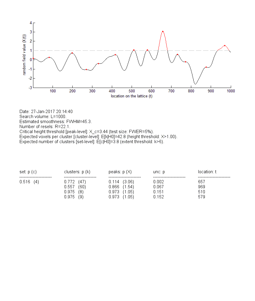
Upper panel: The statistical t-field (y-axis) is plotted against time (x-axis). Local peaks are highlighted in red (if the corrected p-value does not reach significance, here: FWER=5%) or in green (if the corrected p-value reaches significance). The same colour-coding applies to upcrossing clusters (for cluster-level inference). Middle panel: RFT analysis summary (essentially: expectations, under the null, of features of the sample field). Lower panel: list of corrected p-values (set-, cluster- and peak- level inferences). NB: the column “location” relates to local peaks.
One can see that, in this example, no peak or upcrossing cluster reaches statistical significance, when properly corrected for multiple comparisons (compare with uncorrected p-values). This is in fact expected, given that we simulated data under the null. Note: all summary statistics are stored in the out structure, and the sampled statistical field is stored in the variable statfield.
Tip: The RFT results can be explored by right-clicking on either local peaks or upcrossing clusters, which provides a summary of corrected and uncorrected p-values!
GLM with missing data
Missing data occur when the value of either the dependent or the independent variables (or both) are unknown or lost. This is an issue because the model cannot be fitted using the usual procedure (cf. missing values in the design matrix of a GLM). VBA relies on the variational Bayesian algorithm to estimate likely values for missing data in addition to fitting the GLM parameters. See the demo: demo_GLM_missingData.m.
Mediation analysis
One may be willing to address questions about how key variables mediate the impact of (controlled) stimuli onto (measured) experimental outcomes. For example, one may want to assess the impact of brain activity onto behavioural outcomes above and beyond the effect of psychophysical manipulations. Statistical models of mediated effects place the mediator variable (\(M\)) at the interplay between the independent variable (\(X\)) and the dependent variable (\(Y\)). In its simplest form, mediation analysis reduces to inference on the following twofold regression model:
\[\left\{ \begin{array}{ll} M = X \beta_1 + e_M \\ Y = M \beta_2 + X \beta_3 + e_Y \end{array} \right.\]where \(e_M\) and \(e_Y\) are model residuals, and \(\beta_{1,2,3}\) are unknown regression coefficients. Typically, there is a mediation effect if the product \(\beta_1 \times \beta_2\) is different from zero.
On the one hand, VBA proposes to approach such mediation analyses from a Bayesian perspective. The latter perspective reduces to a bayesian model comparison, whereby one evaluates the evidence in favour of a model that includes a serial chain of causality (\(X \rightarrow M \rightarrow Y\)) against a “common cause” model (\(X \rightarrow M\) and \(X \rightarrow Y\)).
On the other hand, VBA comprises self-contained routines for performing classical tests of mediation (e.g., Sobel tests). In brief, this consists in testsing for the significance of the product of path coefficients in the serial model above. Such test can be performed using VBA’s function mediationAnalysis0.m (see the demo: demo_mediation.m).
The following script demonstrates VBA’s GLM classical test functionality:
n = 32; % data sample size
X = randn(n,1); % independent variable
M = X + randn(n,1); % mediator variable
Y = M + X + randn(n,1); % dependent variable (partial mediation)
out = mediationAnalysis0(Y,X,M,[]);
where out is a structure containing the summary statistics of mediation analysis. These are laid out in the matlab command window:
Date: 26-Jan-2017 14:37:13

-- Regression results --
step 1) regress Y on X: R2=0.7% (p=0.65361)
step 2) regress M on X: R2=12.6% (p=0.045935)
step 3) regress Y on both X and M:
   - X: R2[adj]=22.5% (p=0.0070265)
   - M: R2[adj]=58.2% (p=6.1066e-07)

-- Path analysis --
Indirect effect X->M->Y: R2=7.3% (Sobel test: p=0.047847)
Direct effect X->Y: R2=22.5% (p=0.0070265)
Total effect: R2=7.6%
Summary: no conclusion (no X->Y link in the absence of M)

-- Monte-Carlo sampling --
Indirect effect X->M->Y: P(ab=0|H0)=0.03746

-- Conjunction testing --
Indirect effect X->M->Y: P(ab=0|H0)=0.045935
with the following graphical output:
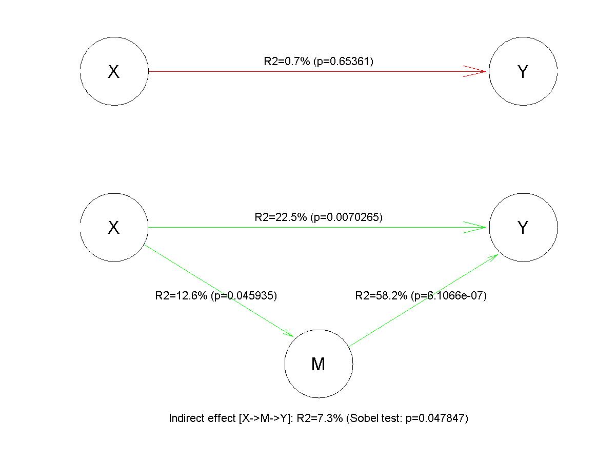
One can see that the direct regression of \(Y\) onto \(X\) (in the absence of the mediatior \(M\)) yields no significant result. However, the full model captures the partial mediation effect.
Tip: Note that mediation analyses of this sort can be generalized to multiple contrasts on experimental factors, where \(X\) is now a full design matrix with more than one independent variable. In this case, one may want to ask whether \(M\) mediates the effect of any linear combination of independent variables on \(Y\). This can be done using the function
mediation_contrast.m.
Binary data classification
Strictly speaking, VBA’s default generative model copes with continuous data, for which there is a natural distance metric. Now if the data is categorical, there is no such natural metric, and one has to resort to probability distributions dealing with discrete events. For example, binary data can be treated as binomial (Bernouilli) samples, whose sufficient statistic (first-order moment) is given by the observation function. An interesting application is binary data classification. In the linear case, the observation mapping reduces to a linear mixture of explanatory variables (i.e. features) passed through a sigmoid mapping. In this case, classification formally reduces to logistic regression and VBA can be used to estimate feature weights that generalize over trials.
However, the typical objective of classification is not to perform inference ion feature weights. Rather, one simply asks how well would the classifier predict the label of a new (yet unseen) data point. In particular, one is interested in whether the classfier operates better than chance. The established approach here is to use cross-validation. One first partition the data into “train” and “test” datasets. The former is used to fit the classifier weights (this is called “training the classifier”). An example of this is “leave-one-out” procedures, whereby each data point serves as the test set in turn. So-called “k-fold” partitionings generalize this idea, in that the original sample is randomly partitioned into k equal sized subsets, each of which serves as the test set in turn. The generalization error is derived by comparing the predicted and actual labels of the “test” data, for each test set. Classical inference can then be used to ask whether the number of correct classification could be explained by chance.
VBA possesses an in-built function for classfication, namely: VBA_classification.m. It can be used to perform both classical (p-value) and Bayesian (exceedance probability) inference on classifier accuracy using k-fold cross-validation approaches. The following script demonstrates VBA’s GLM classical test functionality:
% simulate binary data
n = 32; % data sample size
p = 10; % number of features
F = randn(n,p); % feature matrix
b = 1+randn(p,1); % feature weights
e = randn(n,1); % additional noise
y = sig(F*b+e)>0.5;
% classify data using default set-up
sparse = 0; % sparse mode
[posterior,out,all] = VBA_classification(F,y,n,1,[],sparse);
where sparseis a flag that can be used to perform sparse estimation of classifier weights.
Let us eyeball the graphical output of the function VBA_classification.m:
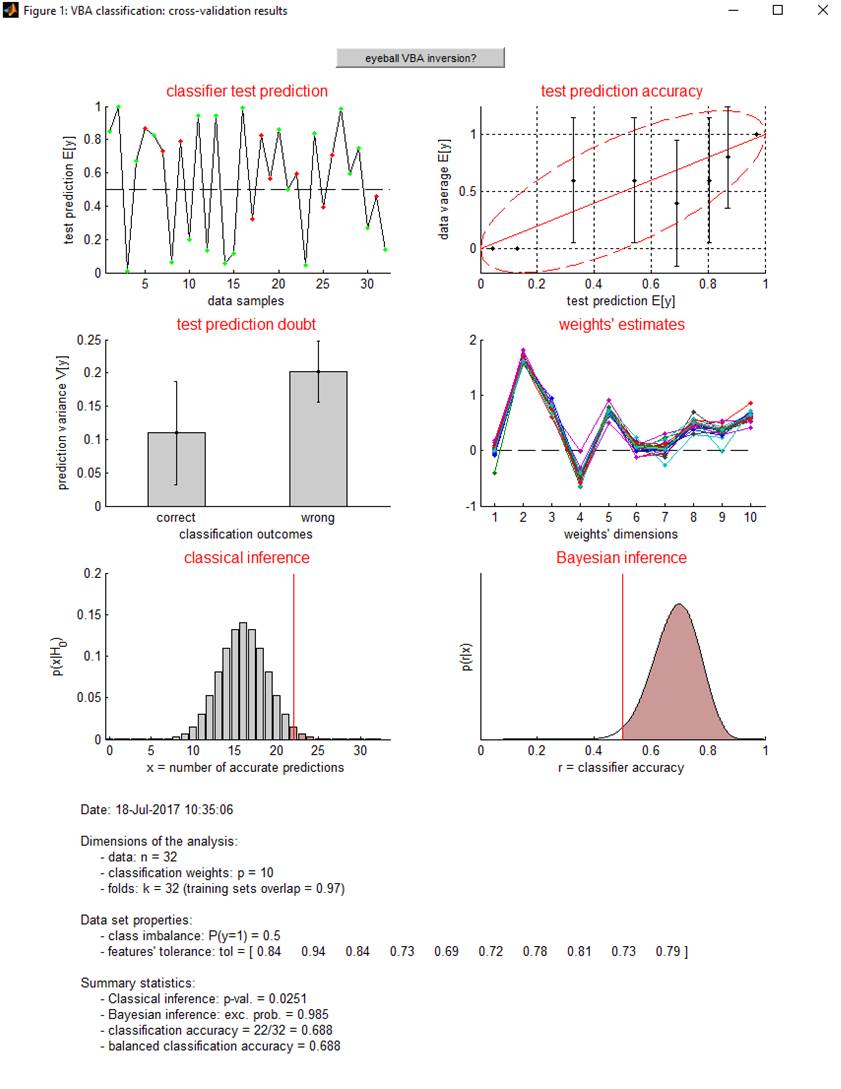
Upper-left panel: classifier test prediction (y-axis) is plotted for all data samples (x-axis), in green (resp. red) if the test classication outcome turned out correct (resp. wrong). Upper-right panel: Data average (y-axis) is plotted as a function of binned classifier test prediction (x-axis). Middle-left panel: classifier test prediction variance is plotted for both correct (left) and wrong (right) classification outcomes. This can be used to evaluate whether test prediction doubt can be used as a proxy for test prediction accuracy. Middle-right panel: classifier weights estimates for each train fold. This can be used to eyeball the estimation stability of classifier weights. Lower-left panel: the distribution of correct classifications (\(X\)) under the null is compared with the actual number of classifier successes (\(x\)). This serves to perform classical inference on classification accuracy: p-value = \(P\left( X>x \mid H_0 \right)\). Lower-right panel: posterior distribution over the classification accuracy. This serves to perform Bayesian inference on classification accuracy (\(r\)): exceedance probability = \(P\left( r>0.5 \mid x \right)\).
One can see on this example that there is no class imbalance, i.e. there is an equal number of \(y=1\) and \(y=0\) observations. Note that class imbalance is not a problem for inference (wheter classical or bayesian) on classification accuracy. However, it may limit the ability of the classifier to generalize on test sets (this would be indexed by a drop in balanced classification accuracy). One can also see that here, classification features are rather uncorrelated (tolerance is always higher than 0.1), which implies that classification weights can be estimated without much identifiability issues.
The script demo_classification.m exemplifies this approach, and demonstrates the relation between classical cross-validation approaches and Bayesian model comparison.
Kalman filter/smoother
A Kalman filter is an algorithm that uses a series of noisy measurements \(y\) observed over time to produce estimates of underlying (hidden) states \(x\) that are assumed to be correlatd over time. In its simplest form, the corresponding generative model is a twofold autoregressive model of the form:
\[\left\{ \begin{array}{ll} y_t = x_t + e_t \\ x_t = x_{t-1} + f_t \end{array} \right.\]where \(e\) and \(f\) are i.i.d. stochastic residuals. The second equation essentially sets a AR(1) prior on hidden states.
The objective of a Kalman filter is to operate on-line and yields an estimate of \(x_t\) given all past observations \(y_{1,2,...,t}\). Alternatively, a Kalman smoother operates off-line, and yields an estimate of \(x_t\) given all observations \(y_{1,2,...,t,...,T}\). This can be useful, because the impact of hidden states may be delayed in time. Lagged Kalman filters provide a reasonable trade-off between the two perspectives, and yield estimates of \(x_t\) given lagged observations \(y_{1,2,...,t,...,t+k}\), where \(k\) is the lag. VBA offers to directly control the backward lag \(k\), by trading computational cost against estimation efficiency.
The script demo_KalmanSmoother.m demonstrates the smoothing properties of the Kalman lagged filter. Here, simulated hidden states follow a triangular wave, whose observation is perturbed with white noise. Critically, we render the inversion scheme blind during half a period of the oscillation. We then invert the model (under AR(1) priors on hidden states), with and without large backward lag.
Probabilistic clustering
Any Bayesian data analysis relies upon a generative model, i.e. a probabilistic description of the mechanisms by which observed data are generated. The main VBA functions deal with a certain class of generative models, namey: state-space models with unknown evolution/observation parameters. But it also offers a set of VB routines developped to invert mixtures of Gaussian -MoG- and of binomial -MoB- densities, which are described below. These can be used to perform data clustering (i.e., blind data classification).
The folder \classification contains the functions that deal with MoG and MoB data (see below).
The MoG model has been widely used in the machine learning and statistics community. It assumes that the observed data \(y\) is actually partitioned into K classes or subsets of points, each one of which can be well described with a multivariate Gaussian density. If these components are sufficiently different, then the overall datasets enjoys a clustering structure, when projected onto an appropriate subspace.
Any arbitrary density over continuous data can be described in terms of a MoG, given a sufficient number of components or classes.
The function VBA_MoG.m inverts, using a variational Bayesian scheme, the MoG model. Given the data \(y\), and the maximum number of classes K, it estimates the most likely number of classes, and the ensuing data labels (as well as 1st- and 2nd- order moments of each Gaussian component). In addition, it also returns the model evidence, which can be useful for model comparison purposes. Running the demo demo_GMM.m would produce the following graphical output of VBA_MoG.m:
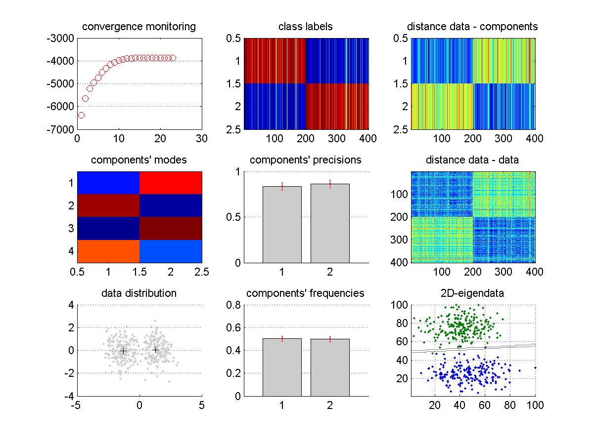
along with the following analysis summary (displayed in the matlab command window):
Initialing components' modes (hierarchical clustering)... OK.
1 component's death: K = 11.
2 component's death: K = 9.
3 component's death: K = 6.
1 component's death: K = 5.
1 component's death: K = 4.
1 component's death: K = 3.
1 component's death: K = 2.
---
Date: 26-Jan-2017 15:08:03
VB converged in 24 iterations (took ~3 sec).
Dimensions:
     - observations: n=400
     - features: p=4
     - modes (final number): K=2
Posterior probabilities:
     - MoG: p(H1|y)= 1.000
     - null: p(H0|y)= 0.000
In this example, 4D data (sample size = 400) was simulated under a MoG model with two components. The inversion started with K=12 components, and eventually removed all unnecessary components (cf. “component’s deaths”). This is called automatic relevance determination or ARD. As in any VBA inversion, convergence monitoring derives from iterative improvements over the model’s free energy, which can be eyeballed on the upper-left panel. Other panels report summary statistics of the relevant posterior densities (including estimated data labels). In addition, the clusters’ separability can be eyeballed on the lower-right panel, which shows an eigen-projection of the data. This projection can be reproduced as follows: VBA_projectMoG(posterior,out,y), with VBA’s output structures.
Now suppose you design an experiment, in which n subjects are asked a number yes/no questions from a questionnaire. Suppose these subjects are grouped into K categories, which are defined in terms of how likely its member are to answer ‘yes’ to each of the questions. You have just defined a MoB model, which you can use to disclose the categories of subjects from their profile of responses to the questionnaire. This is what the function MixtureOfBinomials.m does, using either a Gibbs sampling algorithm or a variational Bayesian algorithm. In both cases, the function returns the data labels, the first- order moment profile for each category and the model evidence. NB: in the MoB case, the inversion schemes cannot automatically eliminate the unnecessary classes in the model. Therefore, (Bayesian) model comparison is mandatory to estimate the number of classes in the data, if it is unknown to the user. See the demo: demo_BMM.m.