Volterra decomposition is a diagnostic analysis that allows one to identify the hidden states’ impulse response to experimentally controlled inputs. This section demonstrates the use of Volterra decompositions in the context of associative learning.

Using inversion diagnostics for refining models

Identifying relevant mechanisms is arguably the most difficult task in modelling complex behavioural and/or biological data. In fact, one may not be in a position to suggest an informed model for the data before the experiment. One solution is then to perform a first model inversion, and then to refine the model based upon inversion diagnostics. In this context, Volterra decompositions of hidden states dynamics may be particularly appropriate.

For example, when modelling how subjects update the value of alternative options given the feedback they receive, one may assume that the learning rate may change over trials. However, one may not know what the determinants of learning rate adaptation are. A practical solution to this problem is to first treat the learning rate as a stochastic hidden state, whose random walk dynamics cannot be a priori predicted. One would then use the VBA inversion of such a model to estimate the learning rate dynamics from, e.g., observed people’s choices. Finally, one could then perform a Volterra decomposition of hidden states dynamics onto a set of appropriately chosen basis functions. Volterra kernels may then provide insights into what in the model can be changed to capture the effect of the inputs onto the learning rate’s dynamics. We will see an example of this below.

Volterra decompositions

Most dynamical systems can be described in terms of input-output relationships, where the output \(x\) is typically a function of the history of past inputs \(u\) to the system. Volterra series allow a decomposition of the input-output transformation, as follows:

\[x_t = w^{(0)} + \sum_{\tau} w_{\tau}^{(1)} u_{t-\tau} + \sum_{\tau_1} \sum_{\tau_2} w_{\tau_1,\tau_2}^{(2)} u_{t-\tau_1} u_{t-\tau_2} +\dots\]

where we have chosen a discrete-time formulation. Here, \(\tau\) is some arbitrary time lag and we have truncated the series (up to second order). First-order Volterra kernels \(w^{(1)}\) capture the linear weight of lagged inputs onto the output. First-order Volterra kernels would be equivalent to impulse response functions, would the system be linear. Second-order Volterra kernels \(w^{(2)}\) capture additional hysteresis effects, whereby the systematic response to some input depends upon the input it received at some other time in the past. For example, systems exhibiting “refractory periods” can be captured using second-order Volterra kernels that cancel the first-order impact of inputs during recovery time. Of course, the equation above can be generalized to situations in which multiple inputs drive the system of interest.

Default Volterra analysis in VBA

When performing dynamical systems’ inversion, the VBA toolbox computes the first-order Volterra kernels of the sampled system’s observable outputs and estimated hidden states and observables, w.r.t. to all inputs. The estimation is performed by the function VBA_VolterraKernels.m, which essentially uses the VBA inversion of the equation above. Importantly, goodness-of-fit metrics (coefficient of determination in the continuous case, and balanced classification accuracy in the binomial case) allows one to evaluate whether the truncated Volterra series faithfully captures the input-output relationship.

The Volterra decomposition is performed under the numerical constraint of a finite lag. Choosing the maximum lag is thus necessarily balancing fit accuracy against estimation efficiency. The default maximum lag in VBA is 16. Setting:

options.kernelSize = 32;

effectively asks VBA to estimate Volterra kernels with a maximum lag of 32 time samples.

In addition, one may want to orthogonalize the inputs prior to the Volterra decomposition. This can be done by setting:

options.orthU = 1;

The inputs are orthogonalized in order, i.e. the second input is orthogonalized w.r.t. the first, the third is orthogonalized w.r.t. the first and the second, etc…

One may also want to detrend inputs. The variable options.detrendU controls the order of a polynomial Taylor series which is removed from the inputs and from the system’s dynamics. For example:

options.detrendU = 3;

will explain away any temporal variability (in the inputs and system’s dynamics), which can be explained by a cubic function of time.

Note that one can perform a Volterra decomposition of the system w.r.t. any arbitrary set of inputs by calling VBA_VolterraKernels.m, having appropriately reset the inputs in out.u. Replacing the estimated kernels in out.diagnostics.kernels allows one to eyeball the new Volterra decomposition from the “kernels” tab (cf. VBA_ReDisplay.m). This can be done as follows:

out.u = u0;
out = rmfield(out, 'diagnostics');
[hf, out0] = VBA_ReDisplay(out, posterior, 1);

This first re-sets the inputs in the out structure with the appropriate set (here, u0). Then, the diagnostics structure is removed from out. Therefore, when called, VBA_ReDisplay derives the Volterra deomcposition w.r.t. u0, instead of u. These will be stored in out0.diagnostics.kernels (but can be eyeballed directly from the graphical results window).

Example

The script demo_dynLearningRate.m demonstrates the above procedure, in the context of the two-armed bandit problem. In brief, an agent has to choose between two alternative actions, each of which may yield positive or negative feedbacks. In our case, we reversed the action-outcome contingency every fifty trials. Below, we describe the analysis steps of the script demo_dynLearningRate.m (and its graphical outputs).

Simulating agent’s choices under a sophisticated learning model

First, a series of choices are simulated, under an agent model that learns both the evolving action-outcome contingencies and their volatility (see Bayesian associative learning models on this page).

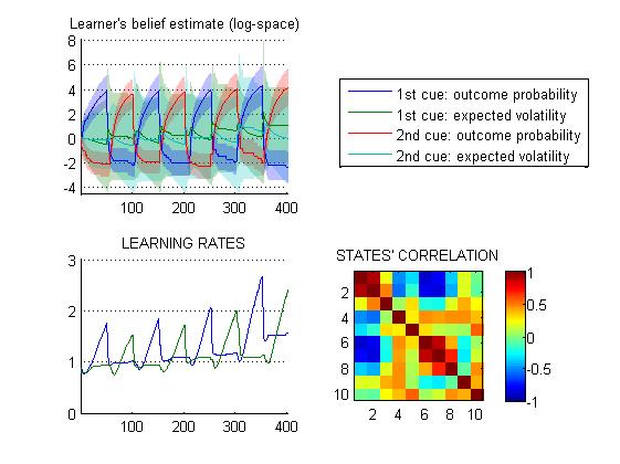
Hidden states of this model include the mean and variance of the agent’s probabilistic belief over the outcome probability and its volatility, given both types of cues (8 states), as well as the outcome’s identity (2 -here, useless- states). One can see how the effective (cue-specific) learning rates evolve over time, as the system’s volatility is inferred from changes in the action-outcome contingencies. In brief, the agent’s inferred volatility increases after each contingency reversal, and then decays back to steady-state.

Inverting a stochastic variant of a Q-learning model

The VBA toolbox is then used to invert a “dynamical” variant of a (much simpler) reinforcement learning model. The only modification to the classical Q-learning model was that the learning rate was allowed to change over time. This was done by augmenting the state-space with a third state that played the role of the learning rate for the first two (native) states. At this point, we are agnostic about how the learning rate should evolve. Thus, its evolution function is set to the identity mapping. Without stochastic state noise, this model is exactly identical to the classical Q-learning model (the learning rate does not change over time, and its value is entirely determined by the -unknown- initial conditions). However, in the presence of stochastic state noise, the learning rate follows a random walk. Unpredictable changes in the learning rate can then be estimated a posteriori, given the agent’s sequence of choices (which was simulated according to a shophisticated hierarchical -volatile- Bayesian learning rule).

Note: the learning rate’s state-noise precision was set hundred time smaller than that of action values. This is to ensure that stochastic deviations from deterministic learning dynamics originate from changes in learning rate (and not in action values). The graphical output of VBA’s inversion of this stochastic variant of the Q-learning model is appended below.

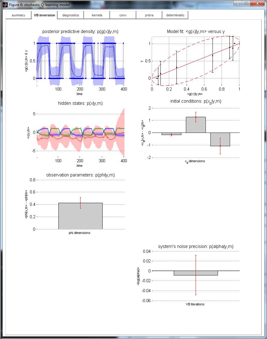
The VBA inversion has identified some variability in the learning rate (cf. posterior estimate of the third states -in red-, on the middle-left graph). A simple classical GLM test allows us to check that this variability correlates with the simulated agent’s inferred volatility (F = 79.2, p<10−8):

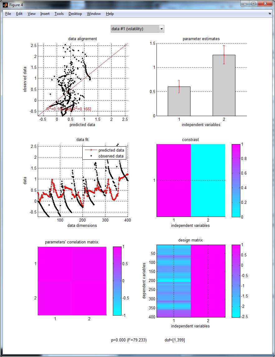
This is the graphical output of GLM_contrast.m, where the design matrix has been set with the simulated agent’s volatility estimate (plus a constant term). See this page for more details regarding GLM_contrast.m.

In brief, the VBA estimate of learning rate time series matches the trial-by-trial simulated agent’s learning rate. This is reassuring, as the problem of estimating learning rates’ stochastic dynamics from observed choices is not a priori trivial.

Performing a Volterra decomposition of learning rates’ dynamics

We then perform a Volterra decomposition w.r.t. three specifically chosen input basis functions, namely: the agent’s last chosen action, the last winning action (which depends upon the outcome and might not be the chosen action), and the winning action instability. The latter is one when the winning action has changed between the previous and the current trial, and is zero otherwise. NB: These three input basis functions can be derived without any knowledge of the underlying learning mechanism. The Q-learner’s choice behaviour is driven by the difference in action values, which mainly responds to the history of winning actions (not shown). In contradistinction, the learning rate exhibits a stereotypical response to winning action instability:

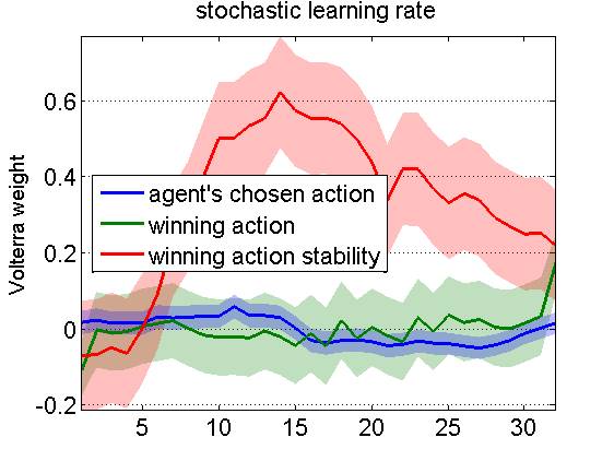
More precisely: following a change in the winning action, the learning rate seems to raise for 15 trials, and then decay back to steady-state in around 20 tials or more. This diagnosis can now be used to augment Q-learning models with deterministic learning rate dynamics, whose impulse response mimic the estimated Volterra kernel.

Refining the generative model based upon Volterra decompositions

An example of the evolution function of such an augmented Q-learning model is given in Daunizeau et al. (2014). In brief, the learning rate’s impulse response to action instability is modelled as a gamma function. Here, two evolution parameters are used, which weigh the impact of the action instability onto the learning rate, and control the decay rate of the impulse response, respectively. Such augmented Q-learning model predicts a transient acceleration of the learning rate following changes in the winning action whenever the weight of the action instability is nonzero. This is confirmed by the VBA inversion of this model:

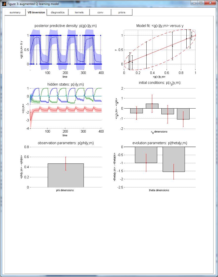
On can see that the deterministic inversion of the augmented Q-learning model exhibits transient changes in the learning rate that appear shorter than those of the stochastic Q-learning model above:

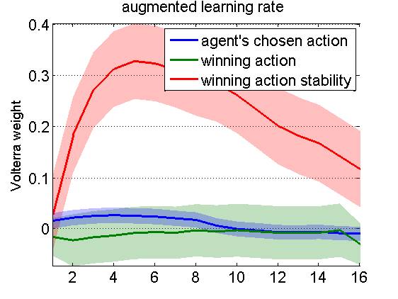
This may be due to the high posterior uncertainty of the learning rate estimates under the stochastic Q-learning model. In fact, Bayesian model comparison yields overwhelming evidence in favour of the augmented Q-learning model, when compared to the standard (but stochastic) Q-learning model.