• Deriving the likelihood function
• Bayes’ rule
• Statistical tests and Bayesian model comparison
• Classical versus Bayesian hypothesis testing

The objective of any data analysis is to discover useful information that can support downstream conlusions and/or decisions. This is trivially true for statistical data analysis, which is typically used to summarize data (cf., e.g., descriptive statistics), or to perform inference (cf., e.g., hypothesis testing). Bayesian data analysis is a specific form of statistical data analysis that relies on so-called generative models, i.e. quantitative scenarios that describe how data were generated. These are used to interpret the observed data, effectively operating “model-based” data analysis. What follows is essentially a crash course on Bayesian inference. We sacrifice a little mathematical rigour for simplicity, in the hope of providing a didactic overview.

Deriving the likelihood function

One usually starts with a quantitative assumption or model of how observations \(y\) are generated. Without loss of generality, this model possesses unknown parameters \(\vartheta\), which are mapped through an observation function \(g\):

where \(\epsilon\) are model residuals or measurement noise. If the (physical) processes underlying \(\epsilon\) were known, they would be included in the deterministic part of the model. Typically, we thus have to place statistical priors on \(\epsilon\), which eventually convey our lack of knowledge, as in “the noise is small”. This can be formalized as a probabilistic statement, such as: “the probability of observing big noise is small” (and, reciprocally: “the probability of observing small noise is big”). It follows that the probability density function of such “small” noise should be bell-shaped (with most of its mass on small values of \(\epsilon\), and decaying quickly for large values of \(\epsilon\)). At this point, one could assume that the noise follows a normal distribution, simply because it provides a parametric form for bell-shaped probability densities:

where \(\sigma\) is the noise’ standard deviation (it determines how big is “big”) and \(m\) is the so-called generative model. Note that \(\sigma\) is often called a hyperparameter, because it determines the expected reliability of the data (see below). Combining the two equations above yields the likelihood function \(p(y\mid\vartheta,\sigma,m)\), which specifies how likely it is to observe any particular set of observations \(y\), given the unknown parameters \(\vartheta\) of the model \(m\) :

This derivation of the likelihood function can be generalized to any generative model \(m\), whose parameters \(\vartheta\) simply control the statistical moments of the likelihood \(p(y\mid\vartheta,m)\). The key point here is that the likelihood function always derives from prior assumptions about observation mappings \(g(\vartheta)\) and measurement noise \(\epsilon\).

Note: There is a slightly more formal justification of the normality assumption (on errors \(\epsilon\)), namely: the principle of maximum entropy. In brief, if one only knows the 1st- and 2nd- order moments of the error, then the normal density is the least informative assumption one can make…

Bayes’ rule

The likelihood function is the statistical construct that is common to both frequentist (classical) and bayesian inference approaches. However, bayesian approaches also require the definition of a prior distribution \(p(\vartheta\mid m)\) on model parameters \(\vartheta\), which reflects knowledge about their likely range of values, before having observed the data \(y\). Such priors can be (i) uninformative (e.g., flat), (ii) principled (e.g. certain parameters cannot have negative values), (iii) conservative (e.g. “shrinkage” priors that express the assumption that parameters are small), or (iv) empirical (e.g., based on previous, independent measurements).

The specific issue of setting the priors is partially adressed here.

Combining the priors and the likelihood function allows one, via Bayes’ Theorem, to derive the posterior probability density function \(p(\vartheta\mid y,\sigma,m)\) over model parameters \(\vartheta\):

where the denominator does not depend upon \(\vartheta\). This is called “model inversion” or “solving the inverse problem”. The posterior density quantifies how likely is any possible value of \(\vartheta\), given the observed data \(y\) and the hyperparameter \(\sigma\) (under the generative model \(m\)). It can be used to extract parameter estimates, e.g. the posterior mean \(E\left[\vartheta\mid y,\sigma,m\right]\), which minimizes the expected mean squared error. Note that here, the hyperparameter \(\sigma\) controls the trade-off between the likelihood and the prior. In brief, if \(\sigma\) is small, then posterior parameters estimates will rely more heavily on the data \(y\) (and less on the prior).

In fact, this dependency can be considered problematic, e.g., if one only has partial knowledge about \(\sigma\). Proper Bayesian inference on model parameters then proceeds by marginalizing hyperparameters out, as follows:

where \(p(\sigma\mid m)\) is one’s (potentially vague) prior belief on \(\sigma\). By construction, the marginal posterior density \(p(\vartheta\mid y,m)\) does not depend upon \(\sigma\) anymore. This approach is in fact very general. In brief, Bayesian inference on “interesting” model parameters (say \(\vartheta\)) always derives from marginalizing “nuisance” parameters (say \(\sigma\)) out.

This approach extends to situations in which one wants to compare models, as opposed to estimate model parameters. Bayesian model comparison primarily relies on the “marginal likelihood” \(p(y\mid m)\) (the so-called “model evidence”), which derives from marginalizing all parameters and hyperparameters out of the likelihood function \(p(y\mid \vartheta,\sigma,m)\):

The model evidence \(p(y\mid m)\) quantifies how likely is the observed data \(y\) under the generative model \(m\). Another perspective on this is that \(-\log p(y\mid m)\) measures statistical surprise, i.e. how unpredictable was the observed data \(y\) under the model \(m\). Under flat priors over models, \(p(y\mid m)\) is used for model selection (by comparison with other models that differ in terms of either their likelihood or their prior density). Importantly, the model evidence accounts for model complexity, and thus penalizes models, whose predictions do not generalize easily (this is referred to as “Occam’s razor”). Note that, although model complexity typically increases with the number of model parameters, the latter is a poor proxy of the former. This is because no complexity cost is incurred when introducing parameters that have a negligible impact on data (see below).

Statistical tests and Bayesian model comparison

Typically, as the quantity of available data increases, Bayesian parameter estimates effectively converge to frequentist (e.g. maximum likelihood) estimators. This is because the weight of the prior on any moment of the posterior distribution becomes negligible.

However, this (asymptotic) equivalence does not hold for model comparison. This is important, because model comparison has many applications within a Bayesian framework. For example, when testing whether a parameter is zero, one effectively compares two hypotheses: the “null”, in which the parameter is fixed to zero, against the “alternative”, in which the parameter is allowed to vary.

According to the Neyman-Pearson lemma, the most powerful test to compare such two hypotheses or models is the likelihood-ratio test, i.e.:

where \(K\) is set to control some statistical risk (see below). This motivates the use of model evidences to perform statistical testing (e.g. testing the null) within a Bayesian framework. In fact, the quantity \(BF_{12}\) is known as the Bayes’ factor, and is used whenever one wants to select between two models. Practically speaking, the Bayes’ factor \(BF_{12}\) induces three types of statistical decisions:

• \(BF_{12}>20\): model \(m_1\) is selected
• \(0.05<BF_{12}<20\): no model is selected
• \(BF_{12}<0.05\): model \(m_2\) is selected

The critical thing to note is that the model evidence \(p\big( y\mid m\big)\) is not a simple measure of model fit: there is an inherent penalization for model complexity. This penalization is intimately related to the priors. In brief, a simple model has tight priors: at the limit, the simplest model has no unknown parameters (infinite prior precision). More complex models are equipped with vague priors, which will be updated to a larger extent once the data has been observed. However, this flexibility has a cost: that of confusing noise \(\epsilon\) with variations in the data that are induced by \(g(\vartheta)\). This is called “over-fitting” the data, and results in greater error when extrapolating model predictions. This is exemplified in the figure below:

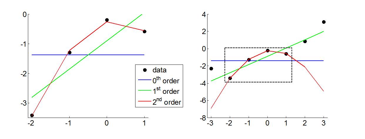
Left: a (noisy) linear model is used to simulate mock data (black dots), which three distinct models are then fitted to: (i) a constant (0th order, in blue), (ii) a linear trend (1st order, in green) and (iii) a quadratic trend (2nd order, in red). Because they do not penalize for model complexity, classical goodness-of-fit measures (e.g., sum of squared residuals) favour the quadratic model over both constant and linear models. Right: model extrapolations are shown, outside the domain of fitted data (dashed balck box). Now any measure of generalization error (e.g., predicted residual error sum of squares or PRESS) would reveal how unreliable the conclusions drawn from the quadratic model were (because of over-fitting). This is a typical situation where classical and Bayesian inference may depart from each other, essentially because the latter would evaluate whether fit accuracy overcompensates the (informational) cost of model complexity.

Model evidence is essentially a trade-off between goodness-of-fit and model complexity. It can be used to compare more than two models, simply because it quantifies the plausibility of the data under any model. In fact, Bayesian model comparison proceeds with the exact same logic as when performing inference on parameters. Here again, one relies upon Bayes’ rule to derive the posterior distribution over models, i.e.:

where \(p(y)\) is the probability of data given all possible models:

The term \(p(m)\) is the prior probability on model \(m\). Typically, non-informative priors are used and the equation above is driven solely by model evidences.

As for any statistical test, a threshold has to be set for deciding whether a model is “better” than another one. This threshold can be chosen similarly to classical statistics, i.e. on the basis of some acceptable decision risk. It turns out that the probability of making a model selection error is \(1-P\left(m^\ast \mid y \right)\), where \(m^\ast\) is the selected model. If this probability has to be controlled at e.g., 0.05, then one “selects” a model only if its posterior probability exceeds 0.95. When comparing two models with each other, this corresponds to a threshold of \(K=20\) on the Bayes’ factor (or, equivalently, 3 on the log- Bayes factor).

This reasoning applies for any set of models, given any data. The only constraint is that model evidences have to be evaluated on the same data set.

Classical versus Bayesian hypothesis testing

Let us first summarize how classical (frequentist) testing proceeds. One starts with defining the null, e.g., some parameter of interest is zero (\(H_0: \theta = 0\)). One then construct a test statistic \(t\) (e.g., Student t-test), for which the distribution under the null \(p\left(t \mid H_0 \right)\) is known. One then evaluates the test statistic given one’s data (\(t^\ast\)) and compare it to the distribution \(p\left(t \mid H_0 \right)\). Typically, one wants to control the false positive rate, i.e. the probability of rejecting the null while it is true. This is why the classical decision rule always look something like this:

CLASSICAL HYP. TESTING: if \(P\left(t>t^\ast \mid H_0 \right) < \alpha\), then reject the null \(H_0\).

This is exemplified in the figure below:

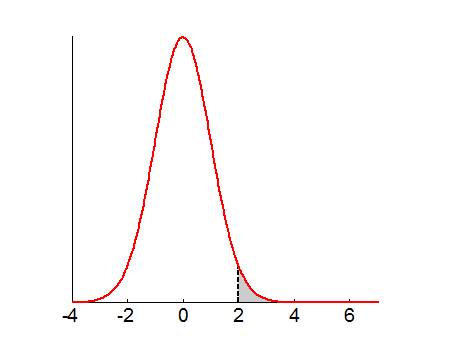
The distribution under the null \(p\left(t \mid H_0 \right)\) is shown in red, along with the probability of finding a more extreme value under the null \(P\left(t>t^\ast \mid H_0 \right)\) (grey area under the curve). Under this decision rule, we expect to wrongly accept the null in \(100 \times \alpha \%\) cases.

But what happens when \(P\left(t>t^\ast \mid H_0 \right) > \alpha\)? Is this evidence in favour of \(H_0\)? Of course not. At this point, one has to resort to the notion of statistical power, i.e. the test’s sensitivity. Formally speaking, sensitivity is one minus the false negative rate, i.e. the probability of not detecting an effect when there is. In principle, this probability can be derived from the alternative hypothesis \(H_1: \theta \neq 0\). For example, if it was the case that, for \(\alpha=0.05\), power was above 95%, then one could be entitled to accept the null, because \(P\left(t < t^\ast \mid H_1 \right) < 0.05\). This logic, however, is more appropriately pursued using Bayesian hypothesis testing.

Recall that Bayesian hypothesis testing is a special case of Bayesian model comparison, whereby one would compare \(H_0\) with \(H_1\). This requires one to consider the alternative hypothesis explicitly. But what novel perspective does it bring? To begin with, although a given data sample may be unlikely under \(H_0\), it may be even more unlikey under \(H_1\). We will see an example of this below. More generally, Bayesian model comparison is more concerned with total error rates than with false positive rates alone. Let us extend our exemple above:

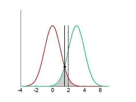
The distribution of possible data samples \(y\) under the null (\(p\left(y \mid H_0 \right)\)) and under the alternative (\(p\left(y \mid H_1 \right)\)) are shown in red and in green, respectively. Under uninformative priors on models, Bayesian model comparison would favour \(H_0\) whenever \(p\left(y \mid H_0 \right) > p\left(y \mid H_1 \right)\), and \(H_1\) otherwise. The ensuing Bayesian decision criterion is depicted using the black solid line, which minimizes the total error rate (grey area under the curve). In this example, Bayesian model comparison would yield more false positives than classical hypothesis testing (cf. dotted black line). However, one can see that this is more than compensated by its higher sensitivity, which yield much smaller false negative rate than classical hypothesis testing.

Note that Bayesian model comparison is not necessarily more liberal than classical hypothesis testing:

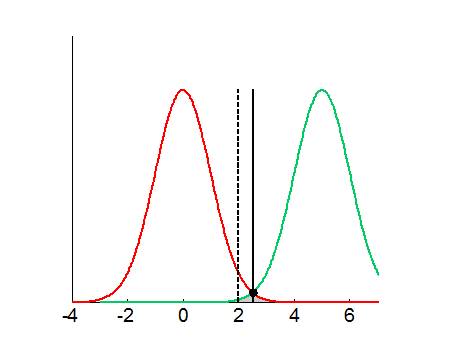
In this example, the alternative hypothesis \(H_1\) is further away from \(H_0\), and Bayesian model comparison would yield less false positives than classical hypothesis testing. Although in this case, Bayesian model comparison would be less sensitive than classical hypothesis testing, its total error rate would still be smaller! This example is in fact typical of situations where, although a given data sample may be unlikely under the null (according to classical hypothesis testing), it may still be even more unlikely under the alternative (cf. data that falls between the classical and the bayesian threshold).

This summarizes why Bayesian and classical hypothesis testing may not yield the same result: the former cares about minimizing total error rates, whereas the latter is obsessed with controlling false positive rates only. In fact, this is the deep reason behind many notorious debates among bayesian and frequentist statisticians, such as, e.g., “Lindley’s paradox“…