WIKI A fast demo: Q-learning
Below, we copied and pasted the content and graphical output of a demonstration script (demo_Qlearning.m) that replicates a typical learning study in behavioural economics and/or experimental psychology.
The task is the so-called two-armed bandit problem, which captures the essence of operant learning. The demo uses the so-called Q-learning model which predicts how people change their behavioural response according to the consequences of their actions (e.g., reward/punishment feedback).
% reformat data
% =========================================================================
% observations
y = choices;
% inputs
u = [ nan, choices(1:end-1)   ;  % previous choice
      nan, feedbacks(1:end-1) ]; % previous feedback

% specify model
% =========================================================================
f_fname = @f_Qlearning; % evolution function (Q-learning)
g_fname = @g_QLearning; % observation function (softmax mapping)

% provide dimensions
dim = struct( ...
    'n', 2, ... number of hidden states (2 Q-values)
    'n_theta', 1, ... number of evolution parameters (1: learning rate)
    'n_phi', 1 ... number of observation parameters (1: temperature)
   );

% options for the simulation
% -------------------------------------------------------------------------
% use the default priors except for the initial state
options.priors.muX0 = [0.5; 0.5];
options.priors.SigmaX0 = 0.1 * eye(2);

% options for the simulation
% -------------------------------------------------------------------------
% number of trials
n_t = numel(choices);
% fitting binary data
options.sources.type = 1;
% Normally, the expected first observation is g(x1), ie. after
% a first iteratition x1 = f(x0, u0). The skipf flag will prevent this evolution
% and thus set x1 = x0
options.skipf = [1 zeros(1,n_t-1)];

% invert model
% =========================================================================
[posterior, out] = VBA_NLStateSpaceModel(y, u, f_fname, g_fname, dim, options);

% compare simulated and estimated model variables
% =========================================================================
displayResults( ...
        posterior, out, choices, ...
        simulation.state, simulation.initial, simulation.evolution, simulation.observation, ...
        Inf, Inf ...
     );
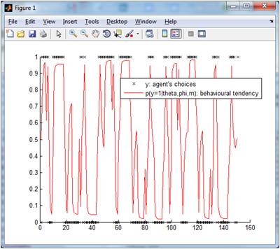
Below are graphical outputs of the demonstration script. First, let us focus on the simulated behavioural tendency and agent’s choices:

One can see how the agent’s behavioural response changes according to the feedback he receives. In brief, the Q-learner is tracking the winning option (which effectively varies over time).
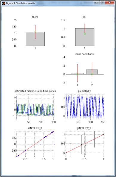
All VBA’s graphical outputs (parameter estimation, model accuracy, inversion diagnostics, convergence, etc…), for this particular example, are described here. Now let us check how accurate the model inversion was (this is the graphical output of displayResults, which is called on the last line of above the demo script):

Upper-left panel: posterior mean (grey bar) and standard deviation (red errorbar) of the model’s evolution parameter (theta = learning rate, here). The simulated parameter is shown using a green dot. Upper-right panel: same for the observation parameter (phi = behavioural log-temperature). Middle-up-right panel: same for initial conditions (options values). Middle-down-left panel: same for hidden states (2 option values plotted as a function of time or trials). Middle-down-right panel: same for observed data. Lower-left panel: estimated hidden states (y-axis) are plotted against simulated hidden states (x-axis). Lower-left panel: fitted data (y-axis) are plotted against simulated data (x-axis).
Recall the unknown parameters of the Q-learning model: 1 evolution parameter (learning rate), 1 observation parameter (temperature) and 2 initial conditions (initial action values). One can see that the posterior credible intervals (red errorbars) contain the simulated parameter values (green dots). In turn, estimated and simulated action values dynamics tightly correlate with each other.
Of course, analysis of experimental data does not allow one to evaluate the accuracy of parameter estimation, as was done here using simulated data. However, VBA provides a number of inversion diagnostics that are useful to review, such as the structure of model residuals, the parameter posterior correlation matrix, Volterra kernels, etc…
If you want to go further, have a look at the demo_QlearningAsymmetric for a more general model (n-armed bandit with asymmetric learning rate).