This page describes the graphical output of the VBA model inversion. In particular, we focus on the example of a Q-learning model given observed choices (see demo_Qlearning.m or this page).

By default, the VBA model inversion terminates by displaying the results in a MATLAB window using tabs, which are described below:

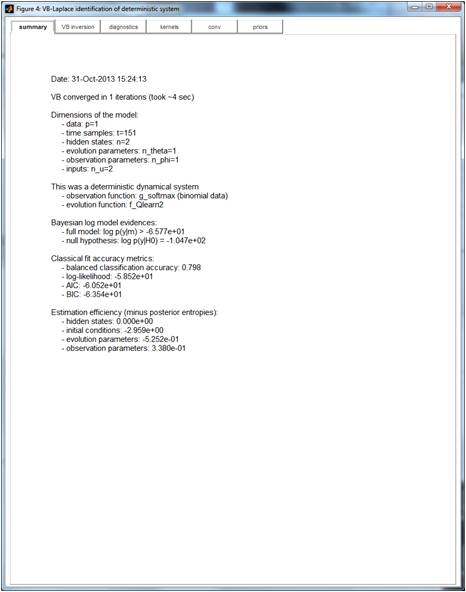
Summary

This tab displays general information about the model inversion, including the log-model evidence for Bayesian model comparison.

TIP: the “null” log-evidence is given here as well, along with fit accuracy metrics (percentage of variance explained, log-likelihood, etc…)

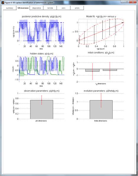
VB inversion

Sufficient statistics of the posterior densities are displayed here (errorbars depict posterior standard deviations, grey barplots show the difference between the posterior and the prior means). These include the posterior predictive densities (which are plotted against time and against data).

TIP: For binary data (as is the case here), the upper-right panel shows the mean and standard deviation of data samples (y-axis) corresponding to six percentiles of the predicted data (x-axis). Ideally, errorbars should align with the red ellipse (along the main diagonal).

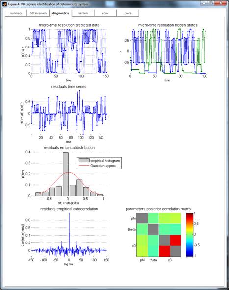
Diagnostics

Diagnostics include estimated state- and measurement noise time-series, noise histograms and autocorrelation, as well as the parameters’ posterior correlation matrix, etc…

TIP: a high posterior correlation between model two model parameters means that they are non-identifiable (they have the same impact on the data). In our example, only the difference between the initial conditions is identifiable (increasing any of these initial conditions has the same effect on data, hence the positive posterior correlation).

Kernels

This tab shows the Volterra decomposition of data and system’s states onto the set of the system’s inputs. Would the system be linear, Volterra kernels would be the impulse response function of the system.

TIP: Volterra weights (y-axis) are plotted against time lag (x-axis) for each input. Positive weights mean that the system’s output increases with the corresponding (lagged) input.

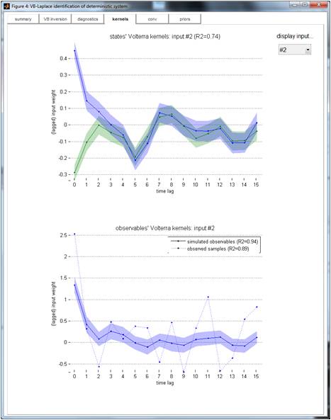
Volterra kernels shown here are those relative to the “winning action” (see VBA’s fast demo), which was encoded as follows: it was 1 when the winning action was the first action, and -1 otherwise. It follows that the first (resp. second) Q-learner’s action value exhibits a positive (resp. negative) exponentially decaying impulse response to the winning action. In the model, the decay rate of the Volterra kernel is simply controlled by the learning rate. Note that the choice is modelled as a binomial variable, whose log-odds is proportional to the difference between the first and second action values. This is why the observables’ Volterra kernel is a positive exponentially decaying function of past winning actions.

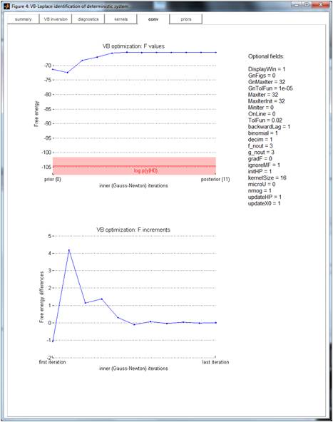
Conv

This is useful for checking the convergence of the VB algorithm. One can eyeball the history of free energy optimization over iterations of the VB algorithm.

TIP: The “null” log-evidence (+/-3) is also shown, for comparison purposes. This provides a dummy Bayesian p-value test for the model (against chance).

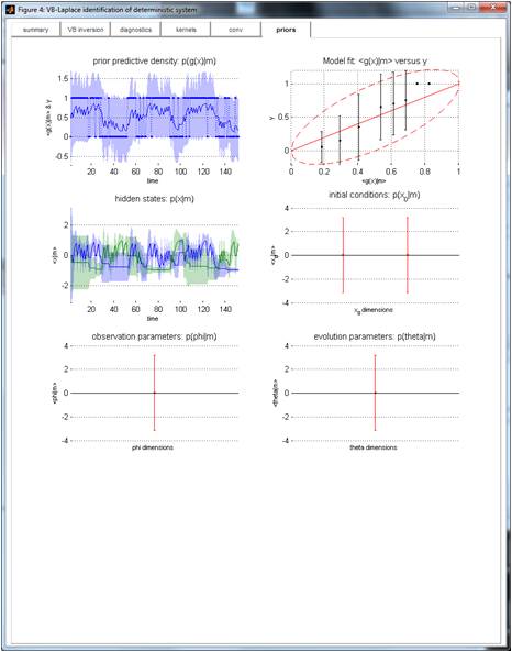
Priors

This tab creates a similar display than ‘VB inversion’, but with the sufficient statistics of the prior density (including the prior predictive density, which is also plotted against the data).

TIP: this is useful to get an idea of how much was learned during the model inversion (cf. comparison of prior and posterior predictive densities).