WIKI The variational Bayes approach

• Mean-field approximation
• Laplace’s approximation
• Limitations

This section summarizes the approximate bayesian inference approach, which VBA relies on.

Recall that, typically, generative models have some form of nonlinearity, in the way the unknown model parameters \(\vartheta\) impact the data \(y\). In particular, the ensuing likelihood function may contain high-order interaction terms between subsets of the unknown model parameters (e.g., because of nonlinearities in the model). This implies that the high-dimensional integrals required for Bayesian parameter estimation and model comparison cannot be evaluated analytically. Also, it might be computationally very costly to evaluate them using numerical brute force or Monte-Carlo sampling schemes. This motivates the use of variational approaches to approximate Bayesian inference (Beal, 2003). In brief, variational Bayes (VB) is an iterative scheme that indirectly optimizes an approximation to both the model evidence \(p(y\mid m)\) and the posterior density \(p(\vartheta\mid y,m)\). The key trick is to decompose the log model evidence into:

where \(q(\theta)\) is any density over the model parameters, \(D_{KL}\) is the Kullback-Leibler divergence and the so-called free energy \(F(q)\) is defined as:

where the expectation \(\langle\rangle_q\) is taken under \(q\). One can see that maximizing the functional \(F(q)\) with respect to \(q\) indirectly minimizes the Kullback-Leibler divergence between \(q(\vartheta)\) and the exact posterior \(p(\vartheta\mid y,m)\). The decomposition of the log evidence is complete in the sense that if \(q(\vartheta)=p(\vartheta\mid y,m)\), then \(F(q)=\ln p(y\mid m)\).

The iterative maximization of free energy is done under simplifying assumptions about the functional form of \(q\), rendering \(q\) an approximate posterior density over model parameters and \(F(q)\) an approximate log model evidence (actually, a lower bound). VBA relies on two such approximations, which we quickly review below.

Mean-field approximation

So what sort of simplifying assumptions can be used to render the VB algorithm computationally and statistically and efficient? A possibility here is to neglect some of the interdependencies between unknown model variables. Typically, one first partitions the model parameters \(\vartheta\) into distinct subsets and then assumes that \(q\) factorizes into the product of the ensuing marginal densities. This assumption of “mean-field” separability effectively replaces stochastic dependencies between model variables by deterministic dependencies between the moments of their posterior distributions:

where \(K\) is a normalization constant and we have used a bi-partition of the parameter space (\(\vartheta=\big\{\vartheta_1,\vartheta_2\big\}\)). Critically, the equation’s right-hand term can be broken down into a weighted sum of the moments of the distribution \(q(\vartheta_2)\). This means that one can update the moments of \(q(\vartheta_1)\) from those of \(q(\vartheta_2)\), and reciprocally. The equation above can be generalized to any arbitrary mean-field partition and captures the essence of the variational Bayesian approach. The resulting VB algorithm is amenable to analytical treatment (the free energy optimization is made with respect to the moments of the marginal densities), which makes it generic, quick and efficient.

Laplace’s approximation

In addition to the mean-field trick, VBA relies upon a further parametric approximation, which essentially consists in summarizing the marginal posterior distributions in terms of their two first-order moments (mean and variance). This effectively operates a local Gaussian approximation to the marginal posterior densities:

where the mean \(\mu_1\) and the variance-covariance matrix \(\Sigma_1\) are given by:

Here, \(I_1\left(\vartheta_1\right) = \langle \ln\:p(\vartheta\mid m) + \ln(y\mid \vartheta,m)\rangle_{q(\vartheta_2)}\) is termed the “variational energy” of \(\vartheta_1\) (it derives from the above mean-field approximation). Typically, any optimization scheme can be used to find the first-order moments of the marginal densities (VBA uses a modified Gauss-Newton scheme). The second-order moments are then obtained by evaluating the local curvature of variational energies. Taken together, mean-field and Laplace approximations are known as the variational-Laplace approach to approximate Bayesian inference (Friston et al. 2007).

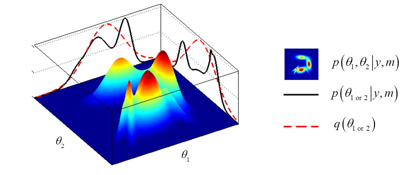
In this mock example, the bidimensional landscape is the (unknown) true joint posterior distribution over both model parameters. The mean-field approximation essentially summarizes this landscape in terms of the product of the respective marginal distributions (cf. black plain lines). Under the Laplace approximation, these marginal distributions further simplify into Gaussian densities (cf. red dotted lines).

The statistical properties of the variational-Laplace approach (e.g., in terms of the quality of the ensuing approximation), for the class of models considered in VBA, were first described in Daunizeau et al. (2009). Additional mathematical details regarding the variational-Laplace approach can be found in this technical note

Limitations

As one might guess, VBA relies on a combination of the above mean-field and Laplace approximations to perform Bayesian inference. Practically speaking, the interest here lies in that the resulting VB algorithms are much more efficient than sampling-based approaches (such as, e.g., Gibbs sampling, rejection sampling, MCMC, etc). This is important, because slow inference schemes may not, even with the help of modern distributed computing, be applicable for state-of-the-art data analysis.

However, VB algorithms have their drawbacks. Some of these are less problematic than they sound, essentially because one can easily diagnose the issue and find a way around. Below, we list the two main VB limitations, which we think one should be aware of:

• Local optima: VB is an iterative optimization scheme (informed by the Free Energy gradient). As any optimization scheme, it can get stuck in local optima. This may impact on the accuracy of both parameter estimation and model comparison. Fortunately, local optima typically induce some form of under-fitting. Sometimes, under-fitting can easily be diagnosed using fit accuracy metrics (such as percentage of explained variance, which VBA provides). In more subtle cases, one might have to inspect the structure of fit residuals (which can be eyballed from VBA’s graphical outputs). Anyway, in such cases, a simple solution is to re-run the analysis with a different initialization (cf, e.g., so-called “multi-start” algorithms), and use Bayesian Model Averaging …
• Overconfidence: VB typically neglects conditional dependencies, in particular when relying on mean-field approximations. This may yield “overconfident” parameter estimates, i.e. posterior variances may be under-estimated. Diagnosing an overconfidence issue is most often impossible from simple sanity checks on a given model inversion. In brief, it effectively requires a specific type of simulation-recovery analysis, whereby posterior variances are compared to squared estimation errors. An example of such an analysis is given in this paper. In principle, it is always possible to re-parameterize the generative model in order to relax most (if not all) mean-field separability assumptions. This, however, may turn out to be quite cumbersome for VBA beginners…

Now, if you think you face an issue of these (or other) sorts, and do not know how to solve it, then do not hesitate to post your issue on VBA’s forum :)

For a more exhaustive review of VB algorithms and their limitations, please refer to this technical note!