WIKI Bayesian model selection for group studies
- FFX-BMS
- RFX-BMS
- Between-conditions RFX-BMS
- Between-groups RFX-BMS
- A note on model scores: VB Free Eneergy, AIC or BIC?
Here, we address the problem of Bayesian model selection (BMS) at the group level. First of all, note that one could perform such analysis under two qualitatively distinct assumptions:
- fixed-effect analysis (FFX): a single model best describes all subjects
- random-effect analysis (RFX): models are treated as random effects that could differ between subjects, with an unknown population distribution (described in terms of model frequencies/proportions).
Note: In classical statistics, random effects models refer to situations in which data have two sources of variability: within-subject variance and between-subject variance, respectively. The latter is typically captured in terms of the spread (over subjects) of within-subject parameter estimates. This is not equivalent to RFX-BMS, where one assumes that the model that best describes a given subject may depend upon the subject.
We first recall how to perform an FFX analysis. We then expose how to perform a RFX analysis. Finally, we address the problem of between-groups and between-conditions model comparisons. The key idea here is to quantify the evidence for a difference in model labels or frequencies across groups or conditions.
FFX-BMS
In brief, FFX-BMS assumes that the same model generated the data of all subjects. NB: Subjects might still differ with each other through different model parameters. The corresponding FFX generative model is depicted in the following graph:
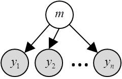 where \(m\) is the group’s label (it assigns the group to a given model) and \(y\) are (within-subject) experimentally measured datasets.
Under FFX assumptions, the posterior probability of a given model is expressed as:
\[p(m\mid y_1,\dots,y_n )\propto p(y_1,\dots,y_n\mid m)p(m)= p(y_1\mid m)\dots p(y_n\mid m)p(m)\]Thus, FFX-BMS simply proceeds as follows:
- for each subject, invert each model and get the corresponding (log-) model evidence,
- sum the log-evidences over subjects (cf. equation above),
- compare models as usual (i.e. as in a single-subject study) based upon summed log-evidences.
FFX-BMS is valid whenever one may safely assume that the group of subjects is homogeneous (i.e., subjects are best described by the same model \(m\)).
RFX-BMS
In RFX-BMS, models are treated as random effects that could differ between subjects and have a fixed (unknown) distribution in the population. Critically, the relevant statistical quantity is the frequency with which any model prevails in the population. The corresponding RFX generative model is depicted in the following graph:
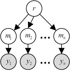
where \(r\) is the population frequency profile, \(m\) is the subject-specific model label (it assigns each subject to a given model) and \(y\) are (within-subject) experimentally measured datasets.
in VBA, the above RFX generative model can be inverted as follows:
[posterior,out] = VBA_groupBMC(L) ;
where the I/O arguments of VBA_groupBMC are summarized as follows:
L: Kxn array of log-model evidences (K models; n subjects)posterior: a structure containing the sufficient statistics (moments) of the posterior distributions over unknown model variables (i.e. subjects’ labels and model frequencies).out: a structure containing inversion diagnostics, e.g.: RFX log-evidence, exceedance probabilities (see below), etc…
In Stephan et al. (2009), we introduced the notion of exceedance probability (EP), which measures how likely it is that any given model is more frequent than all other models in the comparison set:
\(EP_i = P\left(r_i > r_j \mid y\right)\) where \(j\neq i\).
Estimated model frequencies and EPs are the two summary statistics that typically constitute the results of RFX-BMS. They can be retrieved as follows:
f  = out.Ef ;
EP = out.ep ;
Protected exceedance probabilities (PEPs) are an extention of this notion. They correct EPs for the possiblity that observed differences in model evidences (over subjects) are due to chance (Rigoux et al., 2014). They can be retieved as follows:
PEP = (1-out.bor)*out.ep + out.bor/length(out.ep), whereout.boris the Bayesian Omnibus Risk (BOR), i.e. the posterior probability that model frequencies are all equal.
The graphical output of VBA_groupBMC.m is appended below (with random log-evidences, with K=4 and n=16):
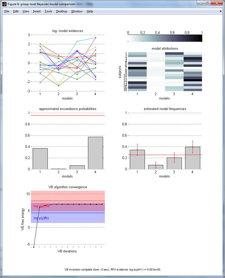
Upper-left panel: log-evidences (y-axis) over each model (x-axis). NB: Each line/colour identifies one subjects within the group. Middle-left panel: exceedance probabilities (y-axis) over models (x-axis). Lower-left panel: RFX free energy (y-axis) over VB iterations (x-axis). The log-evidence (+/- 3) of the FFX (resp., “null”) model is shown in blue (resp. red) for comparison purposes. NB: here, the observed log-evidence are better explained by chance than by the RFX generative model (cf. simulated random log-evidences)! Upper-right panel: model attributions (subjects’ labels), in terms of the posterior probability (colour code) of each model (x-axis) to best explain each subject (y-axis). Middle-right panel: estimated model frequencies (y-axis) over models (x-axis). NB: the red line shows the “null” frequency profile over models.
Optional arguments can be passed to the function, which can be used to control the convergence of the VB scheme.
Importantly, one may want to partition the model space into distinct subsets (i.e. model families). For example, a given family of models would contain all models that share a common feature (e.g., some non-zero parameter). Information Re: model families are passed through the options variable (see header of VBA_groupBMC.m):
options.families = {[1,2], [3,4]} ;
[posterior, out] = VBA_groupBMC(L, options) ;
The above script effectively forces RFX-BMS to perform family inference at the group-level, where the first (resp. second) family contains the first and second (resp., third and fourth) model. Querying the family frequencies and EPs can be done as follows:
ff  = out.families.Ef ;
fep = out.families.ep ;
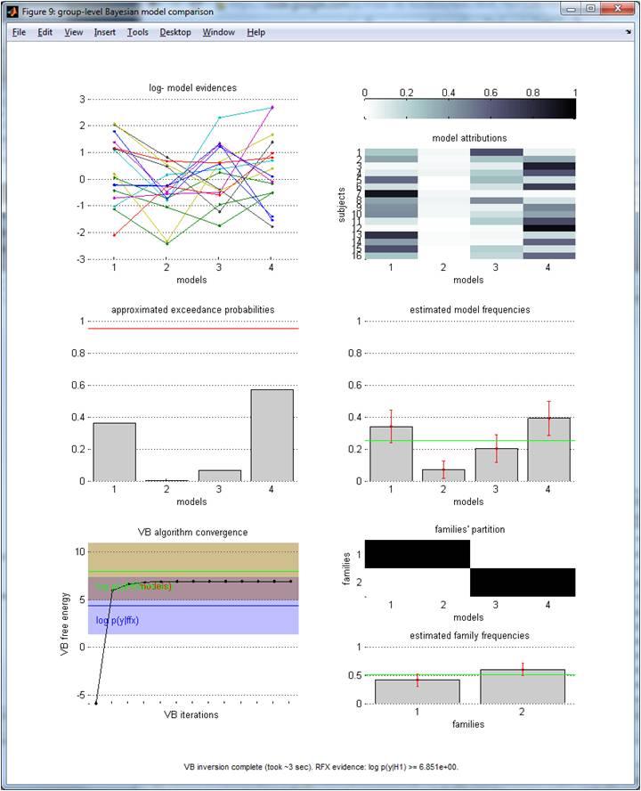
(Same format as before). NB: in the lower-left panel, one can also eyeball the “family null” log-evidence (here, it is confounded with the above “model null”). Lower-right panel: model space partition and estimated frequencies (y-axis) over families (x-axis).
Check demo_modelComparison.m for a more detailed example.
Between-conditions RFX-BMS
Now what if we are interested in the difference between treatment conditions; for example, when dealing with one group of subjects measured under two conditions? One could think that it would suffice to perform RFX-BMS independently for the different conditions, and then check to see whether the results of RFX-BMS were consistent. However, this approach is limited, because it does not test the hypothesis that the same model describes the two conditions. In this section, we address the issue of evaluating the evidence for a difference - in terms of models - between conditions.
Let us assume that the experimental design includes p conditions, to which a group of n subjects were exposed. Subject-level model inversions were performed prior to the group-level analysis, yielding the log-evidence of each model, for each subject under each condition. One can think of the conditions as inducing an augmented model space composed of model “tuples” that encode all combinations of candidate models and conditions. Here, each tuple identifies which model underlies each condition (e.g., tuple 1: model 1 in both conditions 1 and 2, tuple 2: model 1 in condition 1 and model 2 in condition 2, etc…). The log-evidence of each tuple (for each subject) can be derived by appropriately summing up the log evidences over conditions.
Note that the set of induced tuples can be partitioned into a first subset, in which the same model underlies all conditions, and a second subset containing the remaining tuples (with distinct condition-specific models). One can the use family RFX-BMS to ask whether the same model underlies all conditions. This is the essence of between-condition RFX-BMS, which is performed automatically as follows:
[ep, out] = VBA_groupBMC_btwConds(L) ;
where the I/O arguments of VBA_groupBMC_btwConds are summarized as follows:
L: Kxnxp array of log-model evidences (K models; n subjects; p conditions)ep: exceedance probability of no difference in models across conditions.out: diagnostic variables (see the header ofVBA_groupBMCbtw.m).
Now, one may be willing to ask whether the same model family underlies all conditions. For example, one may not be interested in knowing that different conditions may induce some variability in models that do not cross the borders of some relevant model space partition. This can be done as follows:
options.families = {[1,2], [3,4]} ;
[ep, out] = VBA_groupBMC_btwConds(L, options) ;
Here, the EP will be high if, for most subjects, either family 1 (models 1 and 2) or family 2 (models 3 and 4) are most likely, irrespective of conditions.
If the design is factorial (e.g., conditions vary along two distinct dimensions), one may be willing to ask whether there is a difference in models along each dimension of the factorial design. For example, let us consider a 2x2 factorial design:
factors  = [[1,2]; [3,4]] ;
[ep,out] = VBA_groupBMC_btwConds(L, [], factors) ;
Here, the input argument factors is the (2x2) factorial condition attribution matrix, whose entries contain the index of the corresponding condition (p=4). The output argument ep is a 2x1 vector, quantifying the EP that models are identical along each dimension of the factorial design.
Of course, one may want to combine family inference with factorial designs, as follows:
options.families = {[1,2], [3,4]} ;
factors = [[1,2]; [3,4]] ;
[ep, out] = VBA_groupBMC_btwConds(L, options, factors) ;
Note that the ensuing computational cost scales linearly with the number of dimensions in the factorial design, but is an exponential function of the number of conditions (there are K^p tuples).
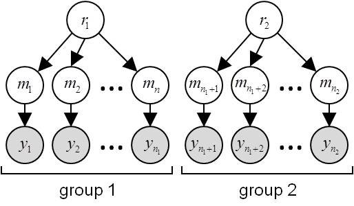
Between-groups RFX-BMS
Assessing between-group model comparison in terms of random effects amounts to asking whether model frequencies are the same or different between groups. In other words, one wants to compare the two following hypotheses (at the group level):
- \(H_=\): data
ycome from the same population, i.e. model frequencies are the same for all subgroups:
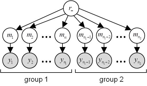
- \(H_{\neq}\): subjects’ data
ycome from different populations, i.e. they have distinct model frequencies:
Under \(H_=\) , the group-specific datasets can be pooled to perform a standard RFX-BMS, yielding a single evidence \(p(y\mid H_{=})\):
L = [L1, L2] ;
[posterior, out] = VBA_groupBMC(L) ;
Fe = out.F ;
where L1 (resp. L2) is the subject-level log-evidence matrix of the first -resp. second) group of subjects, and Fe is the log-evidence of the group-hypothesis \(H_=\).
Under \(H_{\neq}\), datasets are marginally independent. In this case, the evidence \(p(y\mid H_{\neq})\) is the product of group-specific evidences:
[posterior1, out1] = VBA_groupBMC(L1) ;
[posterior2, out2] = VBA_groupBMC(L2) ;
Fd = out1.F + out2.F ;
where Fd is the log-evidence of the group-hypothesis \(H_{\neq}\).
The posterior probability \(P\left(H_= \mid y \right)\) that the two groups have the same model frequencies is thus simply given by:
p = 1/(1+exp(Fd-Fe))
Note that one can directly test for a group difference with the function VBA_groupBMC_btwGroups which directly performs the above analysis:
[h, p] = VBA_groupBMC_btwGroups({L1, L2})
where p is \(P\left(H_= \mid y \right)\).
A note on model scores: VB Free Eneergy, AIC or BIC?
Group-level bayesian model selection (either FFX or RFX) is typically meant to be used with a specific within-subject model scoring metric: namely, the (Bayesian) log model evidence \(\ln p(y\mid m)\). The issue is that, for most generative models, the mathematical derivation of the log evidence is not computationally tractable. If used in conjunction with VBA’s model inversion approach, then one may perform bayesian model selection using VB Free Energies in lieu of models’ log evidences. However, one may also want to use other model scoring metrics, such as AIC (Akaike Information Criterion) or BIC (Bayesian Information Criterion). In fact, VBA automatically computes AIC and BIC (in addition to VB Free Energy). We refer the interested reader to the description VBA’s output. In principle, VB Free Energy, AIC and BIC are all information-threoretic measures of the compromise between fit accuracy (as measured with log likelihood, evaluated at the estimated parameters) and model complexity. They essentially differ w.r.t. the complexity penalty term. So which one should be used?
Formally speaking, VB Free Energy is a lower bound on the model’s log evidence, which makes it an obvious default choice (at least for the advanced VBA user ;)). Similarly, BIC can be regarded as an asymptotic approximation to VB Free Energy (at the limit when the number of parameters is negligible when compared to sample size). This means that, for the purpose of approximating the model’s log evidence, BIC effectively involves additional simplifying assumptions (when compared to VB Free Energy). This is not the case for AIC, which was originally derived under a frequentist inferential framework. But retrospectively, none of these metrics can be deemed a priori better, until some model confusion analysis confirms this for the model selection problem of interest. We suggest the interested reader to have a look at this paper.
Note: AIC and BIC have a sign convention. More precisely, they typically decrease when the data log likelihood increases (i.e. they write something like: A/BIC = -2*log_likelihood + complexity penalty). In VBA, this sign convention is reversed, such that they typically increase with log likelihood (more precisely, both AIC and BIC are multiplied by -2, to make them commensurate to log evidence). This is the proper sign convention, when using AIC or BIC with the above group-level Bayesian model selection approach!