WIKI Behavioural DCM
- Preparing a vanilla DCM analysis
- Setting the neuro-behavioural mapping
- Combining fMRI and behavioural time series
- Running the inversion
- Post-hoc bDCM analysis
Behavioural Dynamic Causal Modelling – or bDCM – aims at decomposing the brain’s transformation of stimuli into behavioural outcomes, in terms of the relative contribution of brain regions and their connections. In brief, bDCM places the brain at the interplay between stimulus and behaviour: behavioural outcomes arise from coordinated activity in (hidden) neural networks, whose dynamics are driven by experimental inputs. Estimating neural parameters that control network connectivity and plasticity effectively performs a neurobiologically-constrained approximation to the brain’s input–outcome transform. In other words, neuroimaging data essentially serves to enforce the realism of bDCM’s decomposition of input–output relationships. In addition, post-hoc artificial lesions analyses allow us to predict induced behavioural deficits and quantify the importance of network features for funnelling input–output relationships. In turn, this enables one to bridge the gap with neuropsychological studies of brain-damaged patients.
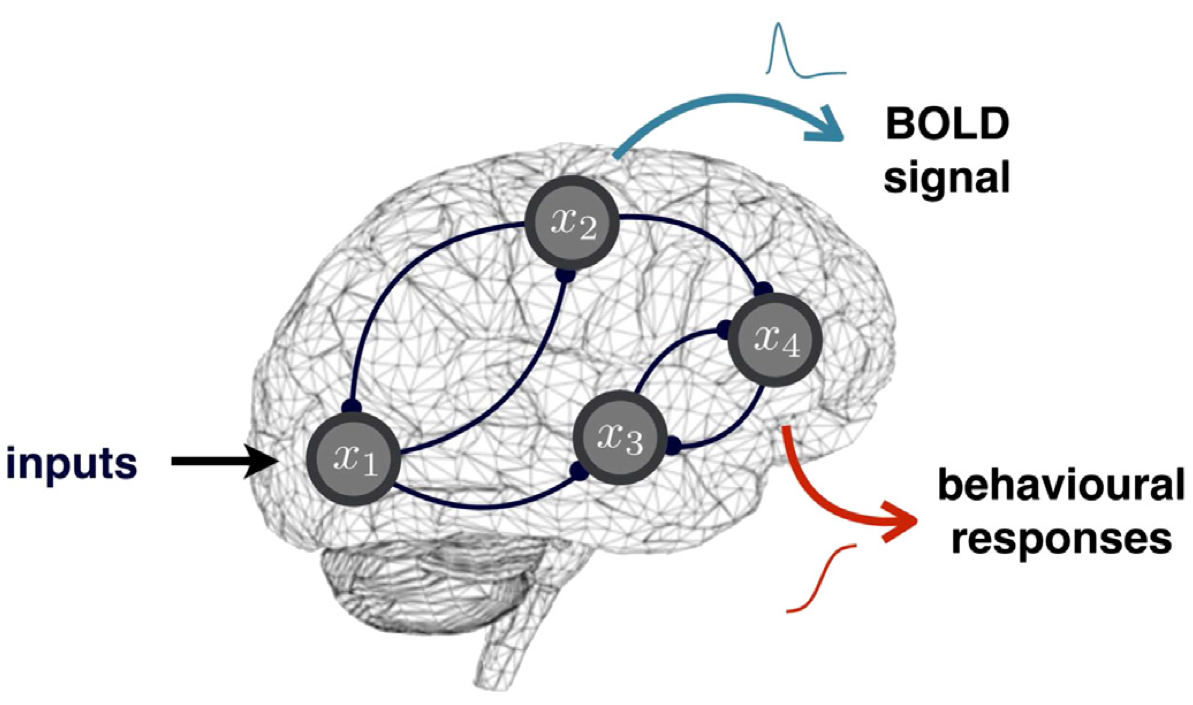
We refer the interested reader to Rigoux & Daunizeau (2015), Dynamic causal modelling of brain–behaviour relationships, Neuroimage 117: 202-221.
What follows is a practical guide to performing a bDCM analysis on your own dataset.
Preparing a vanilla DCM analysis
Recall that vanilla DCM describes how network nodes influence each other using an ordinary differential equation, which is parameterized using \(A\), \(B\), \(C\) and \(D\) matrices. These correspond to connection strengths, input modulations of connections, input-state couplings and state modulations of connections, respectively.
The core steps of a bDCM analysis are identical to vanilla DCM. In particular, you will need to:
- extract fMRI times series
y_fmriin your regions of interest - specify your inputs \(u\)
- setting the DCM connectivity structure (cf. \(A\), \(B\), \(C\) and \(D\) matrices)
We refer the reader to the DCM wiki for more detailed explanations on how to prepare a vanilla DCM analysis using VBA.
Setting the neuro-behavioural mapping
In addition to network dynamics, bDCM augments the state space of vanilla DCM with hidden behavioural predictor variables \(r\) that obey its own set of ordinary differential equations:
\[\frac{dr}{dt}= A_r x + \sum_i u_i B_r^{(i)}x + C_ru + \sum_j x_j D_r^{(j)}x - \alpha r\]where \(A_r\), \(B_r\), \(C_r\) and \(D_r\) matrices define the so-called neuro-behavioural mapping (see below).
You do not have to create an evolution function that implements bDCM hidden states dynamics. This is because VBA already possesses a built-in function that does exactly this, namely:
f_DCMwHRFext.m. This function agregates the evolution function of vanilla DCM with the above behavioural predictor variables dynamics. In addition, VBA also includes dedicated functions that were designed to facilitate the preparation of bDCM analyses. These are described below.
By construction, the behavioural predictor variable \(r\) actually controls the first-order moment of observed behavioural outcomes \(y_{behaviour}\), i.e.:
\[E[y_{behaviour}] = g_r(r)\]where \(g_r\) is some arbitrary observation mapping. Note that the default bDCM observation function in VBA was developed for binary choices (cf. g_DCMwHRFext.m); in this case, \(g_r(r)=\frac{1}{1+e^{-r}}\) is a simple sigmoidal mapping.
In bDCM, all variables (including \(A\), \(B\), \(C\), \(D\), \(A_r\), \(B_r\), \(C_r\) and \(D_r\) matrices) are jointly estimated from both fMRI and behavioural time series. And as in vanilla DCM, users must specify the model structure, which reduces to indicating which entries of these matrices are non-zero. We will exemplify this below. In what follows, we focus on how to set the neuro-behavioural mapping.
Direct neural mapping
The most intuitive part of the neuro-behavioural mapping is a linear predictor that directly maps DCM nodes to behavioural predictors:
Such a linear mapping can be defined through the matrix \(Ar\) that specifies which node can impact on each behavioural response (columns=nodes, lines=responses):
% 2 behavioural responses: r1 is influenced by node 2, and r2 is influenced by node 3
Ar = [ 0 1 0 ;
       0 0 1 ] ;
Modulated neural mapping
Brain-to behaviour mappings may change according to experimental conditions (which are encoded in inputs \(u\)):
Such modulatory effects can be defined through the cell-array \(Br\) that specifies which node-to-response link is modulated by each input in turn (similarly to the \(B\) matrix of vanilla DCM):
% r1 is predicted by the 3rd node modulated by the 2nd input
Br{2} = [ 0 0 1 ;
          0 0 0 ] ;
Direct input-to-output mapping
One may also consider direct influences of inputs onto behavioural responses:

Although it seems counter-intuitive to assume that the impact of experimental manipulation may bypass brain activity, this may provide a useful reference point for assessing the evidence for mediated effects.
This type of “direct mapping” is set through the \(Cr\) matrix:
% r1 is predicted by a linear mixture of the first and second inputs
% r2 is predicted by the last input only
Cr = [ 1 1 ;
       0 1 ] ;
Quadratic neural mapping
Finally, similarly to DCM’s quadratic gating effects, one may assume that brain-to behaviour mappings may be modulated by activity in other network nodes. This captures situations in which nodes interact to produce a response:
These nonlinear effects can be defined through the cell-array \(Dr\) that specifies which node-to-response link is modulated by each node in turn (similarly to DCM’s \(D\) matrix):
% the link from node 3 to r2 is modulated by activity in node 1
Dr{1} = [ 0 0 0 ;
          0 0 1 ] ;
Combining fMRI and behavioural time series
We assume that you have stored the fMRI time series in y_fmri (see how to prepare a vanilla DCM analysis). The full observation matrix y should also include the behavioural observations (choices, reaction times, subjective ratings, pupil responses, etc.) y_behaviour. This might be more tricky than it looks as the multiple sources of observations are usually recorded at different sampling rates. We refer the reader to this page for details regarding this sort of mixed observations.
Now, VBA only deals with one observation function to map hidden states to observed data. Therefore, we need to create an augmented observation function predicting fMRI and behavioural data concurrently. For a vanilla DCM, VBA already provides an observation function: g_HRF3.m. This will be the first ingredient of our (augmented) mixed observation function. The second element is a specific mapping of the behavioural response predictors \(r\). Now if you have a DCM with 3 nodes and 2 behavioral (e.g., button) responses, the mixed observation function should look something like this:
function g = mybDCM(x,P,u,in)
% my dummy bDCM 'augmented' observation function
xdcm = x(1:end-2); % vanilla DCM states (everything except the 2 last states)
g_fmri = g_HRF3(xdcm,P,u,in); % predicted fMRI response (vanilla DCM observation function)
xb = x(end-1:end); % 2 last states = behavioural response predictors (r1 and r2)
g_buttonResp1 = g_myMapping1(xb(1),P,u,in); % dummy r1 mapping
g_buttonResp2 = g_myMapping2(xb(2),P,u,in); % dummy r2 mapping
% mixed fMRI/bhavioural prediction is a 5-elements vector:
g = [g_fmri         ; % 3 lines for the 3 nodes
     g_buttonResp1  ; % r1 (e.g., left hand button press)
     g_buttonResp2] ; % r1 (e.g., right hand button press)
end
where g_myMapping1 and g_myMapping2 can be defined arbitrarily. Such an observation function can be saved and wrapped with appropriate input/output standards (see this page for a complete description of the I/O structure of VBA observation/evolution functions).
Note that bDCM response predictors \(r\) are continuous and unbounded variables. So how do we deal with, e.g., choice data, which are binary? The simplest solution in this case is to use a sigmoid function, like
g_softmax4decoding.m, that will transform \(r\) into the probability of choosing, e.g., the first alternative… In fact, VBA already includes a default bDCM observation function,g_DCMwHRFext.m, that does exactly this. It will apply the vanilla DCM model to the first \(n\) observations (where \(n\) is the number of nodes), and treat all the remaining lines in the data matrix as binary behavioural responses (i.e. in this case, \(g_r\) is the sigmoid mapping). If you want to implement another brain-to-behaviour mapping (that deals with, e.g., continuous responses), you will have to adaptg_DCMwHRFext.maccordingly.
Running the inversion
In VBA, a generative model is defined in terms of an evolution function, an observation function, and a set of priors (see this page for a complete description of the class of VBA’s generative models). VBA already includes generic bDCM’s evolution and observation. All one has to do is to tell VBA about the above connectivity and neuro-behavioural mapping matrices. As for vanilla DCM, the following matlab script creates the corresponding VBA’s options structure:
%- prepare the DCM structure
TR = 2; % sampling resolution (in secs)
microDT = 1e-1; % micro_resolution = ODE solver time step (in secs)
homogeneous = 1; % are all nodes similar?
options = prepare_fullDCM(A,B,C,D,TR,microDT,homogeneous,Ar,Br,Cr,Dr);
Priors can be automatically set using the getPriors function:
nreg = 3; % number of network nodes
n_t = 720; % number of fMRI time samples
reduced_f = 1; % simplified HRF model
stochastic = 0; % for deterministic DCM
options.priors = getPriors(nreg,n_t,options,reduced_f,stochastic);
Note that we may need to inform VBA Re: how to split the observations into fMRI and behavioural time series. The motivation for doing this is twofold: (i) we may want VBA to adapt to distinct signal-to-noise ratios (this can be done by separating fMRI and behavioural data into different “sources”), and (ii) behavioural data may be non-gaussian (e.g., binary). This can be done using the options structure, as follows (for further details, see mixed observations):
% specify distribution of observations
% - three BOLD timeseries / nodes (gaussian)
options.sources(1) = struct('out',1:3,'type',0);
% - two binary behavioural responses (binomial)
options.sources(2) = struct('out',4,'type',1);  % r1
options.sources(3) = struct('out',5,'type',1);  % r2
The main VBA inversion routine can now be called to run the bDCM analysis:
f_fname = @f_DCMwHRFext; % bDCM evolution function
g_fname = @g_DCMwHRFext; %  % default bDCM observation function
dim=options.dim;
[posterior,out] = VBA_NLStateSpaceModel(y,u,f_fname,g_fname,dim,options);
You can have a look at the demo script demo_negfeedback.m that simulates the simple two-nodes bDCM analysis described in our seminal paper (Rigoux & Daunizeau, 2015):
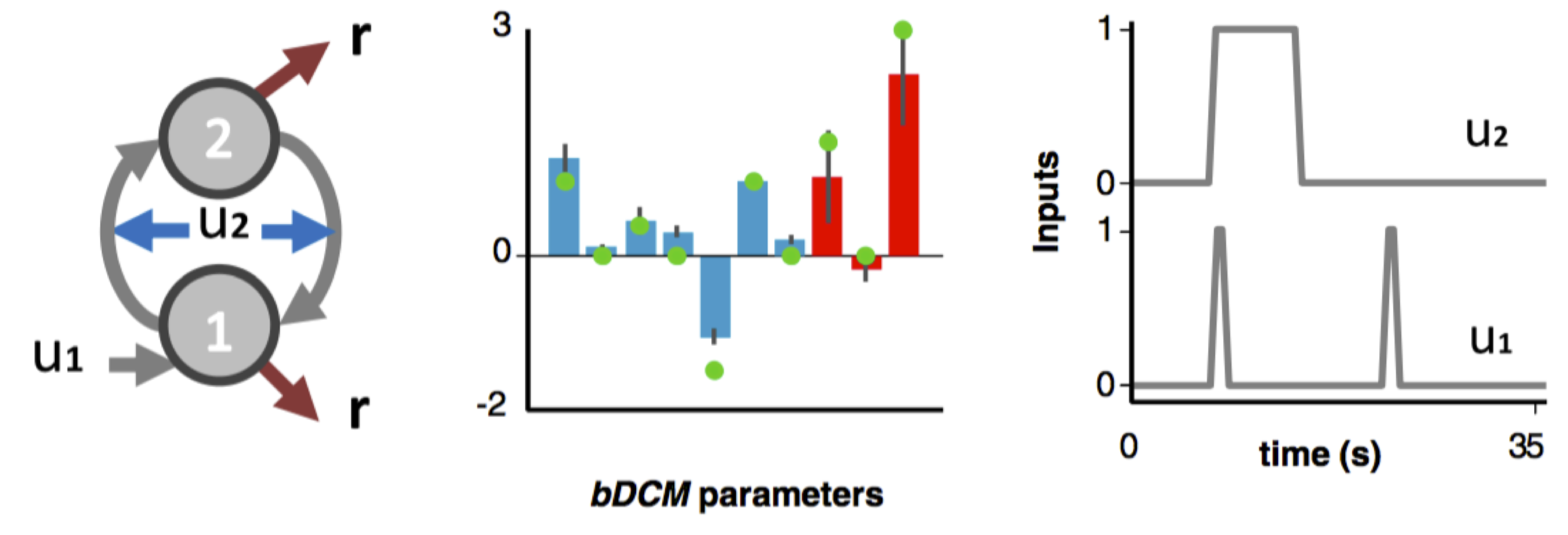
Toy bDCM example from Rigoux & Daunizeau, 2015 The 1st input evokes responses through the action of node 1. The 2nd input modulates the influence of the negative feedback loop formed between nodes 1 and 2.
Post-hoc bDCM analysis
Once the bDCM model has been inverted given mixed fMRI/behavioural times series, one can then perform post-hoc analyses on the model. The objective here is twofold: (i) predict behavioural deficits that would arise from (artificial) lesions on either nodes or links within the network, and (ii) quantify the importance of network nodes or links for funnelling the impact of inputs onto behavioural outputs. As we will se below, VBA is equipped with specific tools for performing these two types of post-hoc analyses.
Artificial lesion analyses
One of the main advantage of bDCM is its ability to predict the effect of brain lesions or dysconnectivity on behavioural responses. To do so, one simply needs to “switch off” the corresponding node or link, simulate the ensuing lesioned model, and summarize the predicted behavioural responses.
In VBA, you can automatically test the effect of lesioning each network node in an automatic manner using the built-in function VBA_bDCM_lesion.m, as follows:
% posterior & out structures come from @VBA_NLStateSpaceModel
results = VBA_bDCM_lesion(posterior, out);

% behavioural timeseries predicted when node 2 is lesioned
results.lesion(2).y
One can then summarize the predicted behavioural responses under different artificial lesions (e.g., node 1 versus node 2) and under different experimental conditions (e.g., distinct values for input \(u_2\)):
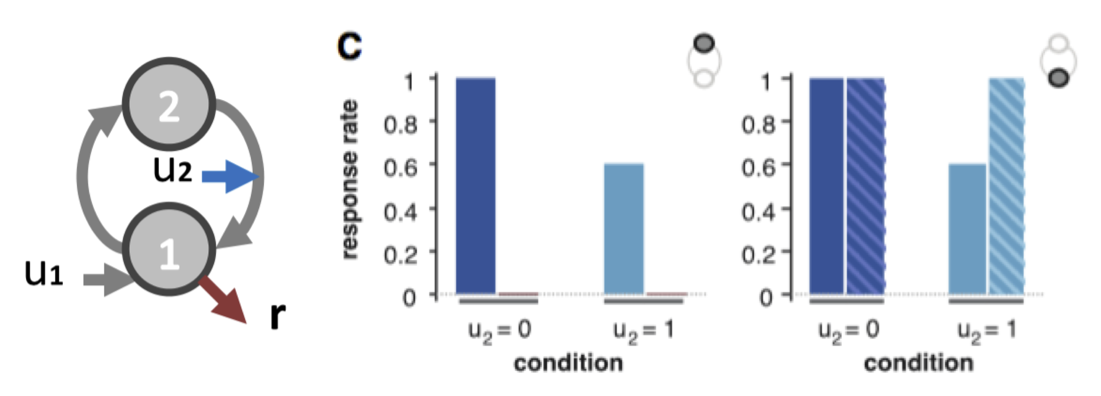
Example of lesion analysis If the 1st node is lesioned (left), then the normal behaviour (plain bars) is completly abolished (hatched bars). If the 2nd node is lesioned (right), we observe an increase in the response rate when the modulatory input is on, showing the loss of feedback inhibition (net effect of connection from node 2 to node 1).
Note that you may want to go beyond such “simple” artificial lesion analysis. In particular, you may be interested in disclosing non-trivial pairwise region-by-region interactions. This may be interesting in the presence of functional redundancy. For exemaple, lesioning a region X alone may not produce any behavioural deficit. The same with region Y. But it may be that if both X and Y are lesioned, then a behavioural deficit is observed. This type of region-by-region may be highly relevant when attempting to related bDCM post-hoc analyses to the neuropsychological studies on brain-damaged patients!
Susceptibility analysis
One may also want to ask which node and/or link is critical for funelling the impact of each input onto each behavioural output. This can be done using so-called “susceptibility analyses”.
Critical here is the fact that measuring the behavioural distortion induced by removing a node or a link is not sufficient for measuring how important is that node or link. This is because one has to account for potential functional redundancy in the system. In brief, if a given input can bypass this node or link to impact behavioural responses, then the corresponding input-output relationship is weakly susceptible to this node or link. We can measure this by measuring the additional additional distortion induced by switching off the input, having already removed the node/link. The amount of additional distortion directly measures functional redundancy. This is because if switching off the input induces additional distoritions, then this means that it did not have to flow through the corresponding node/link… The logic of such analysis is summarized below:
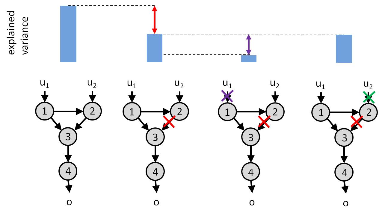
Amount of explained variance in observed behavioural responses (top row) as a function of artificial esions performed on the network (bottom row). Left: un-lesioned network. Lesioning the link from node 2 to node 3 induces a loss of explained variance (red). Further switching off input \(u_1\) induces an additional loss of explained variance (violet). This is because input \(u_1\) can bypass the missing link to impact the behavioural response \(o\) (by flowing directly through node 3). In contrast, switching off input \(u_2\) (green) doesn ot induced any additional loss of explained variance. This is because input \(u_2\) has no other route to pass through. In conclusion, the link from node 2 to node 3 is critical for funneling the impact of input \(u_2\) onto behavioural response.
In VBA, this can be performed automatically using the function VBA_susceptibility, as follows:
% posterior & out structures come from @VBA_NLStateSpaceModel
results = VBA_susceptibility(posterior,out);

% scoring results for each input (line) and connection (column)
results.susceptibility.norm
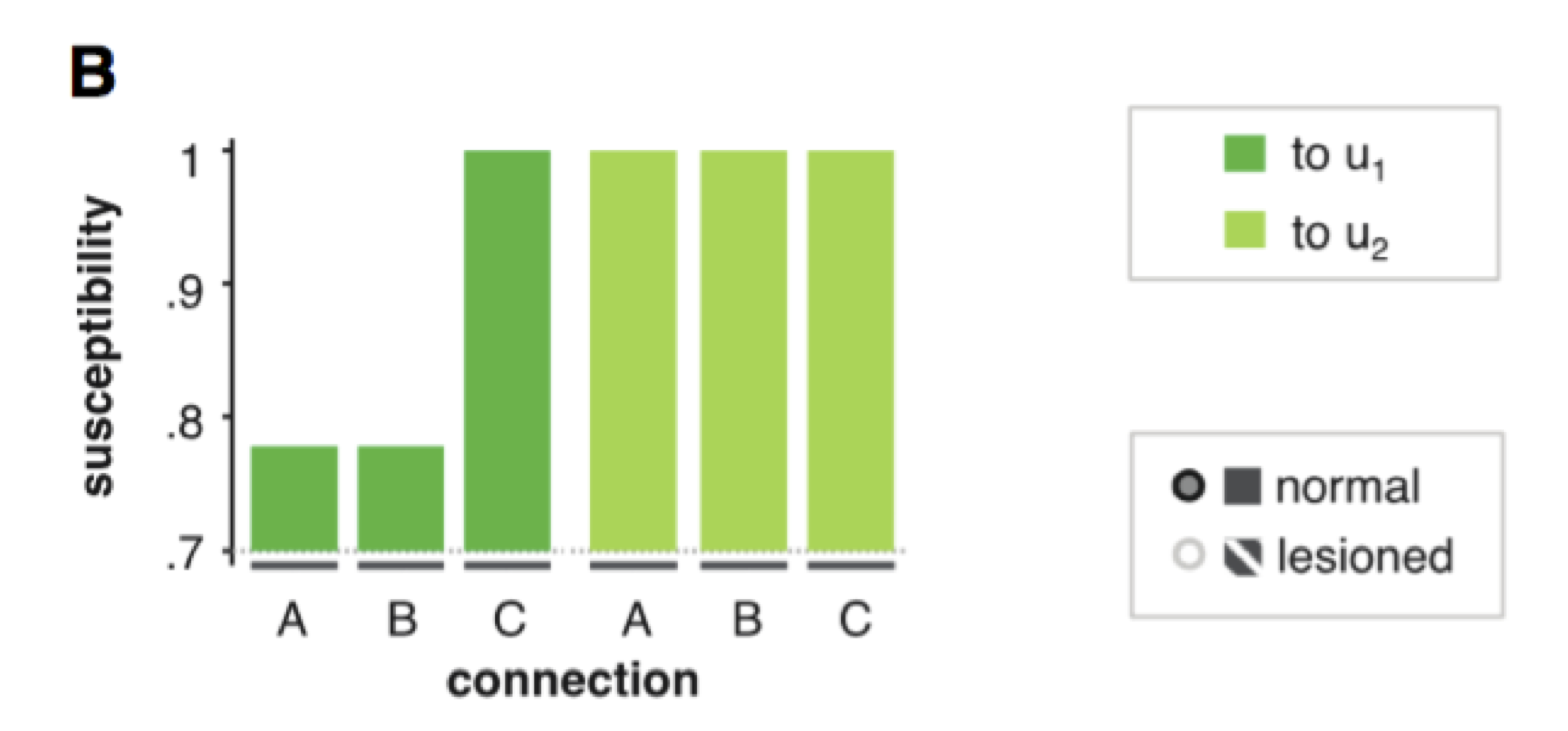
Example of susceptibility analysis. The first input is mostly dependent on parameter \(C\) in our example above, which scores the impact of input \(u\) onto node 1. The modulatory influence of the second input onto the behavioural response requires the two network connections (\(A\) and \(B\)) forming the feedback loop.