This section exposes the structure of generative models that underpin VBA data analysis. But let us start with a simple example.

Example: Q-learning model

Reinforcement learning models are typically used to interpret changes in behavioural responses that arise from subject’s exposure to reward and/or punishment. Among these, Q-learning models simply assume that subjects update the value of possible actions. In its simplest form, the Q-learning algorithm expresses the change in value \(Q_{t+1}-Q_t\) from trial \(t\) to trial \(t+1\) as being linearly proportional to the reward prediction error. This yields the following learning rule:

\[Q_{t+1} = Q_t + \alpha (r_{t+1}-Q_t)\]

where \(r_t\) is the reward delivered to the subject at trial \(t\), and \(\alpha\) is the (unknown) “learning rate” of the subject.

One usually complements Q-learning with a softmax decision rule, i.e. an equation that expresses the probability \(P_t(a_i)\) of the subject to choose action \(a_{i}\) at trial \(t%.\):

\[P_t(a_i) = \frac{\exp \beta Q_t(a_i)}{\sum_j \exp \beta Q_t(a_j)}\]

where \(\beta\) is the (unknown) inverse “temperature”.

Given a series of experienced reward \(r_{t}\) at each trial, these equations can be used to predict the choices of the subject. Fitting the above Q-learning model to behavioural data means finding estimates of the learning rate \(\alpha\), the inverse temperature \(\beta\), and the initial values \(Q_{0}\) that best explains the observed choices (see this page for a demonstration).

Although they are not general enough to capture the range of models that VBA can deal with, these equations convey the basic structure of learning and/or decision making models. This is because:

any form of learning (including probabilistic - bayesian - belief update), can be written as an evolution equation, similar in form to the first equation above
any form of decision making can be understood as an action emission law, and thus written as an observation mapping (from internal states to actions), similar in form to the second equation above.

More generally, most computational models for neurobiological and behavioural data share the same structure, i.e. are based on evolution and/or observation mappings that capture the response of relevant “states” (e.g. neural activity, beliefs and preferences, etc…) to experimentally controlled inputs. We will now describe the general structure of these models in more details.

Nonlinear state-space models

VBA deals with a very general class of generative models, namely: “nonlinear state-space models”. These are reviewed below.

Definitions & Notations

Let us first recall the notations that are used in VBA:

\(y\): experimentally measured data. These can be categorial or continuous. In the Q-learning example above, data are composed of the sequence of observed trial-by-trial choices.
\(x\): hidden states. These are time-dependent model variables, and their dynamics is controlled by the evolution function (see below). In the example above, hidden states are the value of each accessible action.
\(\theta\): evolution parameters. These determine the evolution function of hidden states. In the example above, the only evolution parameter is the learning rate.
\(\phi\): observation parameters. These determine the observation mapping. In the example above, the only observation parameter is the inverse temperature.
\(u\): experimentally controlled inputs. In the example above, the inputs are the reward delivered to the subject.
\(m\): so-called generative model. This encompasses all statistical assumptions that subtend the analysis. In the example above, the generative model includes both learning and decision making equations, as well as priors on model parameters (see below).

The goal of the statistical analysis is to derive both the posterior density \(p(x,\theta,\phi\mid y,m)\) and the model evidence \(p(y\mid m)\). The former quantifies the amount of information one possesses about unknown model parameters, and the latter is used for model comparison.

Evolution and observation mappings

We consider so-called “state-space models”, which essentially consist of two mappings:

The evolution function \(f\) describes how hidden states change from one time sample to the next: \[x_{t+1}=f(x_t,u_t,\theta)+\eta_t\] where \(\eta_t\) are stochastic perturbations, which VBA supposes to be i.i.d. Gaussian, with mean zero and precision (inverse variance) \(\alpha\). In the example above, the evolution function was given by the Q-learning equation, and the state noise precision was infinite (deterministic dynamics, i.e.: \(\eta \rightarrow 0\)).
The observation mapping \(g\) describes how observed data is generated from hidden states. When dealing with continuous data, the observation equation is given by: \[y_t=g(x_t,u_t,\phi)+\epsilon_t\] where \(\epsilon_t\) are model residuals, which VBA supposes to be i.i.d. Gaussian, with mean zero and precision \(\sigma\). In any case, the observation mapping \(g\) specifies the data likelihood \(p(y_t|x_t,u_t,\phi,m)\). In the example above, the likelihood of observed choices was given by the softmax mapping (categorical data).

The following figure summarizes the model structure:

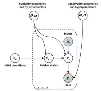
The plate denotes repetitions over time or trials. Nodes represent model variables. Gray nodes represent variables that are known by the experimenter (observed data and controlled inputs). White nodes represent unknown variables (hidden states and parameters of the model). Arrows represent causal dependencies between the variables.

A few specific subcases

Nonlinear state-space models (with unknown evolution, observation and precision parameters) grand-fathers most causal models of the statistical literature. A notable exception are models that include unknown “switch” or categorical variables. We refer the interested reader to this page for an (almost) exhaustive list of generative models that can be emulated using VBA (e.g., auto-regressive models, GARCH models, etc…). Below, we provide two simple specific subcases…

Deterministic dynamical models

One may have to deal with deterministic systems. These simply correspond to the case where the state noise (i.e. the stochastic perturbations of the states’ dynamics) is null (\(\eta=0\)). In this case, the trajectory of hidden states \(x\) through time is entirely determined by inputs \(u\), evolution parameters \(\theta\) and initial conditions \(x_0\). Given the above definition of nonlinear state-space models, determinisic systems arise if you set the priors on the states’ noise precision appropriately (\(\alpha \rightarrow \infty\), see below).

Unless you tell it otherwise, VBA assumes, by default, that your model is deterministic. In fact, even if you change the default prior on the states’ noise precision, VBA initializes the inversion of the (stochastic) model with an inversion of its deterministic variant…

Static models

Note that the above class of generative models encompasses static models, i.e. models without hidden states (nor evolution parameters). In other words, static models simply reduce to a (possibly nonlinear) observation function, i.e.:

\[y_t=g(\phi,u_t)+\epsilon_t\]

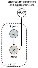
where the observation mapping \(g\) has no notion of “hidden states”. The ensuing graphical model is depicted below:

The simplest variant of all static models is the General Linear Model (GLM), where the observation function \(g\) now reduces to a linear mapping, i.e.:

\[y=X\phi+\epsilon\]

where \(X\) is the so-called design matrix.

In VBA, static models arise if you don’t specify any evolution function. This simpler structure is closer to, e.g., decision making models, whereby subject do not engage in learning. In other terms, there is no need for a temporal structure in decision making models, because there is (typically) no trial-by-trial spillover effect to model…

Prior knowledge

Any data analysis relies upon prior knowledge. For example, the form of the evolution and/or observation mappings is a prior. Within a bayesian framework, the subjective aspect of the inference is made further explicit in the definition of a prior probability distribution \(p(x,\theta,\phi,\alpha,\sigma\mid m)\) over unknown model variables.

Priors can vary in how “informative” they are. This is important because highly informative priors have a strong influence on the posterior. Here, the informativeness is related to how tight the prior probability density is. For Gaussian densities, this is controlled with the covariance matrix (informative = low variance, uninformative = high variance). Note: the contribution of the priors to the posterior tends to be null as the size of data tends to infinity.

\(p(x\mid \theta,\alpha,m)\): priors on hidden states are provided through the form of the evolution function \(f\), which induces a (gaussian) transition probability density \(p(x_{t+1}\mid x_t,\theta,\alpha,m)\) with mean \(f(x_t,\theta,u_t)\) and precision \(\alpha\)
\(p(\theta\mid m)\) and \(p(\phi\mid m)\): priors on evolution and observation parameters are Gaussian distributions that are fully parameterized by their first two moments.
\(p(\alpha\mid m)\) and \(p(\sigma\mid m)\): priors on state and observation noise precisions are Gamma distributions that are fully parameterized by their scale (\(a\)) and shape (\(b\)) hyperparameters. For example, a deterministic system has no state noise \(\eta\), which follows from assuming a priori that \(\alpha\) is 0 with infinite precision \((a_{\alpha}=0\) and \(b_{\alpha}\rightarrow \infty)\).

In brief, the generative model \(m\) includes the evolution and observation functions as well as the above priors on evolution, observation and precision parameters. All these are required to perform a bayesian analysis of experimental data.

In any bayesian data analysis, setting the priors is a subtle issue. Of course, VBA is endowed with “default” priors, which you can change and adapt to your needs (cf. model inversion in 4 steps. Alternatively, VBA enables so-called “empirical Bayes” approaches, e.g. by performing mixed-effect (MFX) modelling…